Locks in Database Management

Previously, you learned about the concurrency mechanism in database. You know that the concurrency is maintained in a serialized manner, giving the impression that there is indeed some concurrency. The locking technique has to do a lot with this achievement of efficient access to database.

What is a Lock?

A lock is a variable associated with a data item that describes the status of the item concerning possible operations that can be applied to it. Accordingly, there is one lock for each data item in the database. Locks are used as a means of synchronizing the access by concurrent transactions to the database item.

Locking protocols are used in database management systems as a means of concurrency control. Many transactions may request a lock on a data item simultaneously. So, we require a mechanism to manage the locking requests made by transactions. Such a  process is called Lock Manager.

It relies on the process of message passing where transactions and lock managers exchange messages to handle the locking and unlocking of data items.

Concurrency control protocols can be broadly divided into two categories −

• Lock based protocols
• Timestamp based protocol

Lock-based Protocols

Database systems equipped with lock-based protocols use a method by which any transaction cannot read or write data until it acquires an appropriate lock on it. Locks are of two varieties:

• Binary Locks − A lock on a data item can be in two states; it is either locked or unlocked.
• Shared/exclusive − This type of locking method differentiates the locks based on their uses. If a lock is obtained on a data item to perform a write operation, it is an exclusive lock.

Allowing more than one transaction to write on the same data item would lead the database into an incompatible state. Read locks are divided because no data value is being changed.

Types of Locks

Several types of locks are used in concurrency control. To implement locking concepts gradually, we need to talk about binary locks, which are simple but restrictive and so are not used in practice.

 After it shared/exclusive locks, which provide more general locking capabilities and are used in practical database locking schemes.

What are Binary Locks?

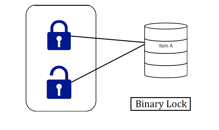
A binary lock can have two states or values locked and unlocked.

A distinct lock is related to each database item A. If the value of the lock on A is 1, item A cannot gain access by a database operation that requests the item.

If the lock value on A is 0 then the item can be accessed when requested. We refer to the current value of the lock associated with item A as LOCK (A).

 There are two operations, lock item and unlock item are used with binary locking A transaction requests access to an item A by first issuing a locked item (A) operation. If LOCK (A) = 1, the transaction is forced to wait. If LOCK (A) = 0 it is set to 1 (the transaction locks the item) and the transaction is allowed to access item A. 

When the transaction is through using the item, it issues an unlock item (A) operation, which assigns LOCK (A) to 0 (unlocks the item) so that A may be accessed by remaining transactions. Hence binary lock imposes mutual exclusion1 on the data item.

Rules of Binary Locks

Incase the simple binary locking scheme described here is used, every transaction must obey the following rules:

• A transaction must supply the operation lock_item (A) before any read_item (A) or write, item operations are performed in T.
• A transaction T must supply the operation unlock_item (A) after all read_item (A) and write_item (A) operations are completed in T.
• A transaction Twill does not supply a lock _item (A) operation if it already holds the lock on Item A.
• A transaction will not issue an unlock _item (A) operation unless it already holds the lock on item A.
• The lock manager module of the DBMS can implement these rules. Between the Lock_item (A) and unlock_item (A) operations in transaction T, is said to hold the lock on item A. 

At most one transaction can hold the lock on a particular item. Thus no two transactions can access the same item together.

Merits of Binary Locks

• They are simple to execute since they are effectively mutually exclusive and establish isolation perfectly.

• Binary Locks request less from the system since the system must only keep a record of the locked items. The system is the lock manager subgroup which is a feature of all DBMSs today.

Disadvantages of Binary Locks

As discussed earlier, the binary locking scheme is too restrictive for database items, because at most one transaction can hold a lock on a given item. So, a binary locking system cannot be used for practical purposes.

One of the methods to ensure isolation of property in the transactions is to require data items to be accessed in a mutually exclusive manner. That means, that while one transaction is accessing a data item, no other transaction can make changes to that data item.

So, the most common method used to implement requirements is to allow a transaction to access a data item only if it is currently holding a lock on that item.

Thus, the lock on the operation is required to ensure the isolation of the transactions.

How Do Shared Locks Function?

• Shared locks survive when two transactions are granted read access.
• One transaction gets the shared lock on data and when the second transaction requests the same data it is also given a shared lock.
• Both transactions are in a read-only mode, updating the data is not allowed until the shared lock is released. There is no difference with the shared lock because nothing is being updated.
• Shared locks last if they need to last; it depends on the level of the transaction that holds the lock.
• Shared locks keep up read integrity. They check whether a record is not in process of being updated during a read-only request.
• Shared locks can also be used to stop any kind of updates of record.
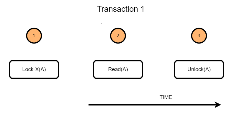
• It is represented by Lock-S which is a read-only lock.
• S-lock is appealed using Lock-S instruction.

Example:

Consider a case where initially A=100 and two transactions are reading A. If one of the transactions wants to update A, in that case, the other transaction would be reading the wrong value.

However, the Shared lock prevents it from updating until it has finished reading!

Exclusive Locks

We should allow several transactions to access the same item A if they all access A’ for reading purposes only. However, if a transaction is to write an item A, it must have total access to A

. For this purpose, a different type of lock called a multiple-mode lock is used. In this scheme, there are exclusive or read/write locks are used.

Example:

Consider a transaction(T2) that requires updating the data item value A. The following steps take place when lock protocol is applied to this transaction.

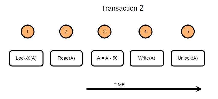
• T2 will acquire an exclusive lock on the data item A
• Read the current value of data item A
• Change the data item as required. In the example illustrated, a value of 50 is subtracted from the data item A
• Write the updated value of the data item
• Once the transaction is finished, the data item will be unlocked.

Differences between Shared Lock and Exclusive Lock

Shared Lock:

• Lock mode is a read-only operation.                                   
• Shared lock can be placed on objects that do not have an exclusive lock already placed on them.
• Prevents others from updating the data.                         
• Provided when the transaction wants to read an item that does not have an exclusive lock.     
• Any number of transactions can hold a shared lock on an item.    
• S-lock is appealed using lock-S instruction.    

Exclusive lock:

• Lock mode is read as well as write operation.
• Exclusive lock can only be placed on objects that do not have any other kind of lock.
• Prevents others from reading or updating the data.
• Provided when transaction wants to update unlocked item.
• Exclusive lock can be observed by only one transaction.
• X-lock is sought using lock-X instruction.

Locking operations

There are three locking operations called read_lock(A), write_lock(A) and unlock(A) represented as lock-S(A), lock-X(A), unlock(A) (Here, S indicates shared lock, X indicates exclusive lock) can be performed on a data item. appealed

A lock related to an item A, LOCK (A), now has three possible states: “read-locked”, “write-locked,” or “unlocked.” A read-locked item is also called a share-locked item because various transactions are allowed to read the item, whereas a write-locked item is caused exclusive-locked. Hence, a single transaction exclusively holds the lock on the item.

Compatibility of Locks

Suppose that there are A and B two different locking modes. If a transaction T1 requests a lock of mode on item Q on which transaction T2 currently holds a lock of mode B.

 If the transaction can be granted the lock, despite the presence of the mode Block, then we say mode A is compatible with mode B. Such a function is shown in one matrix as shown below:

	S	X
S	True	False
X	False	False

The graphs show that if two transactions only read the same data object they do not conflict, but if one transaction writes a data object and another either reads or writes the same data object, then they dispute with each other.

A transaction requests a shared lock on data item Q by executing the lock-S(Q) instruction. Similarly, an exclusive lock is appealed through the lock- X(Q) instruction. A data item Q can be free via the unlock(Q) instruction.

To access a data item, transaction T1 must first lock that item. If the data item is already locked by another transaction in an opposite mode, the concurrency control manager will not allow the lock until all opposed locks held by other transactions have been released. Thus, T1 is made to wait until all opposed locks held by other transactions have been released.

There are four types of lock protocols available are: –

Simplistic Lock Protocol

Simplistic lock-based protocols allow transactions to obtain a lock on every object before a ‘write’ operation is performed. Transactions may unlock the data item after completing the ‘write’ operation.

Pre-claiming Lock Protocol

Pre-claiming protocols estimate their operations and create a list of data items on which they need locks. Before starting execution, the transaction requests the system for all the locks it needs beforehand.

If all the locks are allowed, the transaction executes and releases all the locks when all its operations are over. If all the locks are not allowed, the transaction rolls back and waits until all the locks are granted.

Two Phase Locking 2PL

This locking protocol divides the implementation phase of a transaction into three parts. In the first part, when the transaction starts working, it seeks permission for the locks it requires.

The second part is where the transaction obtains all the locks. As soon as the transaction releases its first lock, the third phase starts. In this phase, the transaction cannot order any new locks; it only releases the acquired locks.

Two-phase locking has two phases, one is increasing, where all the locks are being acquired by the transaction; and the second phase is decreasing, where the locks held by the transaction are being released.

To claim an exclusive (write) lock, a transaction must first obtain a shared (read) lock and then upgrade it to an exclusive lock.

Strict Two-Phase Locking

The first phase of Strict-2PL is the same as 2PL. After obtaining all the locks in the first phase, the transaction continues to execute normally.

 But in contrast to 2PL, Strict-2PL does not release a lock after using it. Strict-2PL holds all the locks until the commit point and releases all the locks at a time.

Strict-2PL does not have to cascade termination as 2PL does.

Timestamp-based Protocols

The most used concurrency protocol is the timestamp-based protocol. This protocol uses either system time or a logical counter as a timestamp.

Lock-based protocols manipulate the order between the conflicting pairs among transactions at the time of execution, whereas timestamp-based protocols start working as soon as a transaction is created.

Every transaction has a timestamp related to it, and the ordering is determined by the age of the transaction. A transaction created at 0002 clock time would be older than all other transactions that come after it. For example, any transaction ‘y’ entering the system at 0004 is two seconds younger and the priority would be given to the older one.

In addition, every data item is given the latest read and write-timestamp. This lets the system know when the last ‘read and write’ operation was performed on the data item.

Timestamp Ordering Protocol

The timestamp-ordering protocol checks serializability among transactions in their conflicting read and writes operations. This is the responsibility of the protocol system that the various pair of tasks should be executed according to the timestamp values of the transactions.

Let’s assume there are two transactions T1 and T2. Suppose the transaction T1 has entered the system at 007 times and transaction T2 has entered the system at 009 times. T1 has the higher priority, so it executes first as it is entered the system first.

The priority of the older transaction is higher that’s why it executes first. To decide the timestamp of the transaction, this protocol uses system time or logical counter.

• The timestamp of transaction T_i is represented as TN(T_i).
• Read time-stamp of data-item X is represented by R-timestamp(X).
• Write time-stamp of data-item X is shown by W-timestamp(X).

Timestamp ordering protocol works as follows −

• If a transaction Ti issues a read(X) operation −

• If TN(Ti) < W-timestamp(X)
  • Operation rejected.
• If TN(Ti) >= W-timestamp(X)
  • Operation executed.
• All data-item timestamps are updated.

• If a transaction Ti issues a write(X) operation −

• If TN(Ti) < R-timestamp(X)
  • Operation rejected.
• If TN(Ti) < W-timestamp(X)
  • Operation rejected and Ti rolled back.
• Otherwise, the operation is executed.

Concurrency control is important in DBMS for handling the simultaneous execution of transactions among various databases.

 Lock Based Protocols being an essential member of the concurrency control technique enforces isolation among the transactions, preserves and maintains the reliability of the database, and resolves the disputes of read-write and write-read operations.

 In addition to Lock-based Protocols, concurrency control can also be achieved via methodologies such as Timestamp Protocol, Multiverse concurrency Protocol, and Validation Concurrency Protocols.

Advantages and Disadvantages of Timestamp Ordering protocol:

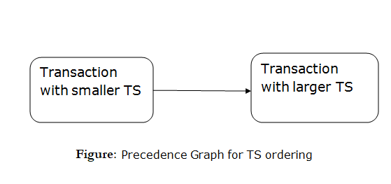
• Timestamp Ordering protocol ensures serializability since the precedence graph is as follows:

• TS protocol ensures freedom from deadlock which means no transaction ever be in waiting.
• But the schedule may not be modified back and may not even be cascade-free.

Summary

You have learned about different types of lock and their efficiencies, drawbacks in this article. The idea of the efficient lock is to maintain faster access and keep the database consistent. This is done when the transaction is kept atomic and isolated.

post

Concurrency Control

The concurrency control concept comes under the Transaction in the database management system (DBMS). It is a procedure in DBMS which helps us control two simultaneous processes to execute without conflicts among every other, these conflicts occur in multi-user systems.

Concurrency explains executing multiple transactions at a time. It is required to increase time efficiency. If many transactions try to access the same data, then irregularity arises. Concurrency control is required to maintain consistent data.

For example, if we take ATMs and do not use concurrency, multiple persons cannot draw money at a time in different places. Hence, we need concurrency.

Advantages

The advantages of concurrency control are: –

• Waiting time will be decreased.
• Response time will gradually decrease.
• It increases Resource Utilization.
• System accuracy & Efficiency is increased.

Control Concurrency

The simultaneous execution of transactions over shared databases can create several data integrity and consistency problems.

For example, if too many people are logging in to the ATMs, serial updates and synchronization in the bank servers should manifest whenever the transaction is done, if not it gives wrong information and wrong data in the database.

Main problems with using Concurrency

The problems which arise while using concurrency are as follows −

• Updates will be lost – If a single transaction does some changes, and another transaction removes that change. One transaction empties the updates of another transaction.

For example:

Consider the below diagram in which two transactions T_X and T_Y, are performed on the same account A where the balance of account A is $300.

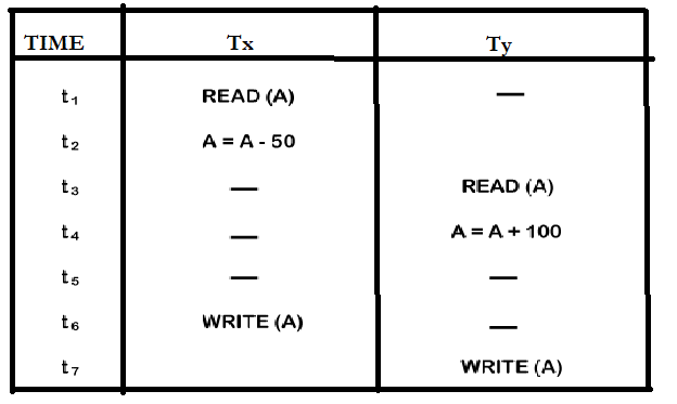
• At time t1, transaction T_X reads the value of account A, i.e., $300 (only read).
• At time t2, transaction T_X deducts $50 from account A which becomes $250 (only deducted and not updated/written).
• Alternately, at time t3, transaction T_Y reads the value of account A that will be $300 only because T_X didn’t update the value yet.
• At time t4, transaction T_Y adds $100 to account A which becomes $400 (only added but not updated/written).
• At time t6, transaction T_X writes the value of account A that will be updated as $250 only, as T_Y didn’t update the value yet.
• Similarly, at time t7, transaction T_Y writes the values of account A, so it will write as done at time t4 which will be $400. Then the value written by T_X is lost, i.e., $250 is lost.

As a result, data becomes incorrect, and database sets to inconsistent.

•  Dirty read problem – The variable which updated in one transaction, at the same time another transaction has started and deleted the value of the variable there the variable is not getting updated or committed that has been done on the first transaction this gives us false values or the previous values of the variables this is a major problem.

For example:

Consider two transactions T_X and T_Y in the below diagram executing read/write operations on account A where the available balance in account A is $300:

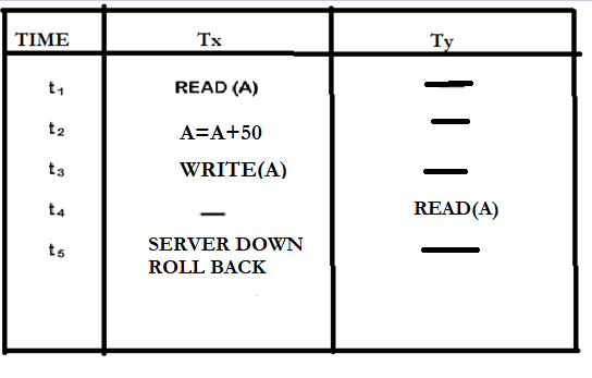
At time t1, transaction T_X reads the value of account A, i.e., $300.

At time t2, transaction T_X adds $50 to account A which becomes $350.

At time t3, transaction T_X writes the newly refurbished value in account A, i.e., $350.

Then at time t4, transaction T_Y reads account A which will be read as $350.

Then at time t5, transaction T_X rollbacks because of a server problem, and the value changes back to $300 (as initially).

But the value for account A remains $350 for transaction T_Y as committed, which is the dirty read and therefore known as the Dirty Read Problem.

Inconsistent retrievals − One transaction is updating multiple different variables, another transaction is in the process to update those variables, and the problem that occurs is the inconsistency of the same variable in various instances.

Concurrency control techniques

The concurrency control techniques are as follows –

Locking

Lock guarantees exclusive use of data items to a current transaction. It first gains the data items by acquiring a lock, after completion of the transaction it releases the lock.

Types of Locks

The variety of locks is as follows: –

• Shared Lock [Transaction can read only the data item values]
• Exclusive Lock [Used for both reading and writing data item values]

Time Stamping

The timestamp is a unique identifier created by DBMS that indicates the relative starting at the time of a transaction. Whatever transaction we are doing stores the starting time of the transaction and denotes a specific time.

This can be created using a system clock or logical counter. This can be implemented whenever a transaction is started. Here, the logical counter in addition after a new timestamp has been assigned.

Optimistic

It is based on the belief that conflict is rare, and it is more efficient to allow transactions to proceed without implementing delays to ensure serializability.

Summary

You are now familiar with concepts of transaction management and concurrency. The concurrency control management of database employs various techniques that ensures that database access smooth and efficient. The concurrency control also makes sure that the database is always in a consistent state.

post

DBMS – Basics

DBMS stands for Database management system is software than help users to access database efficiently. In this lesson you will learn – DBMS Basics

Before DBMS, data was stored in operating system files and each file had its own rules and constraints that required specific applications to access the data.

If the data organization were to change with in the files, then application logic must also change. Sometimes you must write a new application to access the modified data files.

Storing and retrieving of data was very difficult with operating system files. The major disadvantages of these data files are as follows.

Redundancy and Inconsistency

Redundancy means duplicate information. Programmers insert new data or update the data files which leads to redundancy for two reasons.

1. Same information in different files in different format can cause redundancy.
2. Multiple copies of same file is also redundant.

The second problem with the data file is inconsistency. The files are stored in different locations in a different format for different applications, this leads to inconsistency. Updating files concurrently is another reason for the inconsistency.

The cost of accessing the data is also high because applications are written in many programming languages.

Difficulty accessing data

If a user wants some information extracted from data files, we cannot query the flat files directly. As a result, the information must be gathered manually or we have to write an application for that.

There is always a delay associated with the process or retrieving valuable information from data files.

Constraints

Data stored in files must follow some constraints so that it is consistent everywhere in the system.

Suppose, you are working with customer bank accounts and the constraint is to keep the account above $1000. The application has a piece of code that understand this constraint.

If the constraints change then entire application logic must change because the piece of code with the constraint is part of a bigger software program.

Atomicity Problem

If the system fails to record certain data information due to application failure, the database will be inconsistent. Then it is necessary to – Do complete transaction or no transaction at all. This is principle of Atomicity.

If the atomicity is not maintained, then the database will be in an inconsistent state and atomicity is not possible in file-processing systems.

Concurrent Access

There is no system in file-based data storage to maintain concurrent access. If two application users access the same data file – then the update from each concurrent user will not be recorded properly, if both of them write data file at the same time. There is no concurrency control mechanism.

Security Problem

There is no way to access only the relevant part of database files. The application will access all the information it is allowed to access regardless of what it is going to process.

The DBMS on the other hand, load relevant part of the database only.

DBMS Basics – Database system

We know that the DBMS does some amazing things and it is a software product. The core functions of a DBMS can be generalized into following.

1. Database Design
2. Data Analysis
3. Concurrency Control

Complex data structures are hidden and an abstract view of data is presented to users to simplify communication with the database. This is because the technical expertise of users are different.

There are 3 level of data abstraction

1. Physical – At this level the system administrator is user who decide and maintain the physical storage for DBMS.
2. Conceptual – The Database administrator is user at logical level and design, maintain the organization database.
3. External or View – The user at this level at normal users who use the system for other purposes.

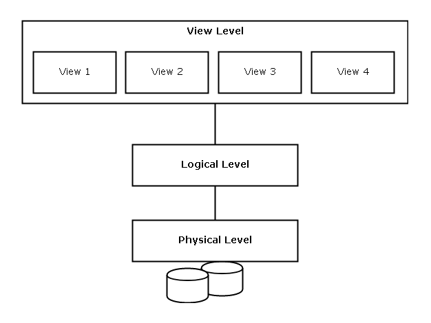
At each level, the user does not need to know the complexity at the level below and this is known as data independence.

Database Schema

Overall design of database is called the database schema. The database schema is very important during the design process. There is a relation between the level of abstraction and database schema.

For example,

• Physical Schema at physical level.
• Logical schema at Logical level
• Schema at view level is sub-schema.

The information stored in database at a particular moment is called instance of database. The instance of database contains collections of records.

Data Model

A data model describe a way to describe the database at physical, logical and view levels. It helps user to store data in terms of data model. These are the main type of data model used in DBMS.

1. Relational Model
2. E-R Model
3. Object-Based data Model
4. Semi-structured Data model

Database Languages

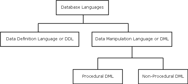
Data-Manipulation Language or DML

DML is the query language and performs some data manipulations. You can divide the DML into two part – Procedural and Non-procedural DML.

The common tasks performed by DML are

1. Insert
2. Delete
3. Update
4. Query

Procedural DML you can define a procedure or function. It defines what to query and how to query. In case of procedural DML, you many require a procedural language. They are hard to write because you need expertise in two languages.

Non-procedural DML also known as Declarative DMLs only define what to query.

e.g,

select * from department;

Data-Definition Language or DDL

Storage structure and access methods in DDL and stored in data dictionary contains metadata information – (data about data.)

e.g. create table, alter table, change a field name or type, etc.

create table department (deptid number (2), deptname varchar2 (15));

DDL for constraints

• Domain constraints – integer, float, etc.
• Referential integrity – attribute in a table must appear in another table (referential integrity). Any change that break this constraint is denied.
• Assertion – a condition that the database must satisfy all the time.

Relational Database

The relational database is made of tables and each table has rows and columns. The tables are also known as relations. The rows are called the tuples and the columns are attributes or fields.

Department Relation

DeptID	DeptName	Location
12	Finance	London
34	Operations	Tokyo

In the DBMS Basics – example above, the columns – DeptID, DeptName and Location are fields or attributes of a Department.

The row with DeptID 12 and 34 are tuples or records of Department table.

References

Avi Silberschatz, Henry F. Korth, and S. Sudarshan. 27-Jan-2010. Database System Concepts. McGraw-Hill Education.

Ramakrishnan, Johannes Gehrke, and Raghu. 1996. Database Management Systems. McGraw Hill Education; Third edition (1 July 2014).

post