Linear Algebra Archives - Page 2 of 3

Inverse Of Matrix

In linear algebra, matrix inverse holds a special place because there is no division in matrix algebra. You cannot divide two matrices. Fortunately, the division is possible when a matrix is multiplied with its inverse which is unique.

The inverse is not possible with just any kind of matrix, a matrix must be square and invertible and the reasons are explained in this article along with several identities and examples involving inverse matrices.

An inverse matrix can also be used for finding the solution for system of linear equations, that is, $Ax = b$ where $A$ is augmented matrix, $x$ is the solution vector and $b$ is the constant vector.

What Is The Need For Inverse?

Inverse means opposite of some operation performed and the result obtained is identity of that operation.

For example,

Additive Identity

If $a + 0 = a$ then $0$ is additive identity.

$3 + 0 = 3$

But,

$3 - 3 = 0$ (additive identity).

Therefore, subtraction is inverse operation of addition.

Multiplicative Identity

If $a \times 1 = a$ then $1$ is multiplicative identity because it gives $a$ as result.

$4 \times 1 = 4$

But,

$4 \times \frac{1}{4} = 1$ ( multiplicative identity).

Therefore, multiplying with reciprocal or division is inverse operation of multiplication.

The same idea can be extended to matrix since we are unable to divide two matrices directly. If $A$ is a square matrix and invertible , then find an inverse matrix $A^{-1}$ such that multiplying it with $A$ will give an identity matrix $I$ of same order.

\begin{aligned} A.A^{-1} = A^{-1}.A = I \end{aligned}

For example,

Let $A$ be a square matrix of order 2 x 2. The inverse of matrix $A$ is $A^{-1}$ .

\begin{aligned} &A = \begin{bmatrix} 2 & 1\\ 2 & 6\end{bmatrix} \end{aligned}

Computer the determinant.

\begin{aligned} &Det(A) = 2\times 6 - 1 \times 2 = 12 - 2 = 10 \end{aligned}

Add negative to following elements in matrix $A$ .

\begin{aligned} A = \begin{bmatrix} 2 & 1\\ 2 & 6\end{bmatrix} = \begin{bmatrix} + & -\\ - & +\end{bmatrix} = \begin{bmatrix} 2 & -1\\ -2 & 6\end{bmatrix} \end{aligned}

Swap positive entries.

\begin{aligned} &\begin{bmatrix} 2 & -1\\ -2 & 6\end{bmatrix} = \begin{bmatrix} 6 & -1\\ -2 & 2\end{bmatrix} \end{aligned}

Multiply the above result with $\frac{1}{det(A)}= \frac{1}{10}$ .

\begin{aligned} &A^{-1} = \frac{1}{10}\begin{bmatrix} 6 & -1\\ -2 & 2\end{bmatrix}\\\\ &= \begin{bmatrix} 3/5 & -1/10\\-1/5 & -1/5\end{bmatrix} \end{aligned}

Let us now verify whether $A.A^{-1} = A^{-1}.A = I$ .

\begin{aligned} &\begin{bmatrix} 2 & 1\\ 2 & 6\end{bmatrix} \times \begin{bmatrix} 3/5 & -1/10\\ -1/5 & -1/5\end{bmatrix}\\\\ &= \begin{bmatrix} 6/5 - 1/5 & -1/5+ 1/5\\ 6/5 - 6/5& -1/5+ 6/5\end{bmatrix}\\\\ &= \begin{bmatrix} 1 & 0\\ 0 & 1\end{bmatrix} \end{aligned}

Why Square Matrix ?

The inverse deals with negative power such as $A^{-1}$ , a non-square matrix is cannot be used because it is undefined( cannot multiply).

The second reason for using square matrix is the identity matrix. An identity matrix is a square matrix only. A product of non-square matrix with its inverse will not result in an identity matrix.

If a square matrix $A$ has inverse matrix $B$ such that

\begin{aligned} &AB = BA = I \end{aligned}

Then the matrix $A$ is called invertible matrix and matrix $B$ is its inverse. If there is no $B$ for matrix $A$ , then it is called Singular matrix.

A matrix is singular and has no inverse if its determinant is 0. You will learn about determinants in future lessons.

Suppose $A$ is a singular matrix of order 2 x 2.

\begin{aligned} &A = \begin{bmatrix}a & b\\c & d\end{bmatrix}\\\\ &ad - bc = 0 \end{aligned}

In the same manner, determinants of higher order matrices is found.

Therefore, only square matrix is used to find inverse which is also a square matrix of size $n \times n$ .

Uniqueness Of Inverse Matrix

If a square matrix $A$ is invertible, then it has exactly one inverse.

Proof :

Suppose that there are two inverse $B$ and $C$ for matrix $A$ . We get

\begin{aligned} &AB = BA = I - (1)\\\\ &AC = CA = I - (2) \end{aligned}

We know that any matrix multiplied by Identity matrix will result itself. Therefore, the following is true.

\begin{aligned} &B = B.I\\\\ &B = B(AC) \hspace{5px}by \hspace{5px}(2)\\\\ &B = (BA)C \hspace{5px}by \hspace{5px}associativity \hspace{5px}property\\\\ &B = I.C \hspace{5px}by \hspace{5px}(1)\\\\ &B = C\\\\ \end{aligned}

Use Of Inverse Matrix

The purpose of using matrix is to solve for $A.x = b$ where $A$ represents the augmented matrix obtained from the system of linear equations, $x$ is the vector of unknowns or solution vector and $b$ is the constant vector.

\begin{aligned} A.x = b => \begin{bmatrix}a & b\\c & d\end{bmatrix}.\begin{bmatrix}x \\ y\end{bmatrix} = \begin{bmatrix}b_1 \\ b_2\end{bmatrix} \end{aligned}

Multiply both sides by $A^{-1}$ . Note that the order of operation is important.

\begin{aligned} &(A^{-1}A)x = A^{-1}b\\\\ &By \hspace{5px} A^{-1}A = AA^{-1} = I, \hspace{5px}we\hspace{5px} get \\\\ &Ix = A^{-1}b => x = A^{-1}b\\\\ \end{aligned}

Let us try to solve a system of equation using above result where $A$ matrix is invertible and square. Suppose the system of equations have following equation.

\begin{aligned} &2x + 4y = 10\\\\ &3x + 2y = 7 \end{aligned}

Let $A$ be a square and invertible augmented matrix of order 2 x 2 derived from the system of equations above. Therefore, $A.x = b$ is as follows.

\begin{aligned} &A.x = b\\\\ &\begin{bmatrix}2 & 4\\3 & 2\end{bmatrix} . \begin{bmatrix}x \\ y\end{bmatrix} = \begin{bmatrix}10 \\ 7\end{bmatrix} \end{aligned}

Let us find the inverse of matrix $A$ . But, first we must find the determinant of matrix $A$ .

\begin{aligned} Det(A) = ad - bc = 4 - 12 = -8 \end{aligned}

Change the sign and swap the positive entries. Then multiply it with $\frac{1}{Det(A)}$ to get the inverse of matrix $A$ .

\begin{aligned} \begin{bmatrix}2 & 4\\3 & 2\end{bmatrix} = \begin{bmatrix}+ & -\\- & +\end{bmatrix} = \begin{bmatrix}2 & -4\\-3 & 2\end{bmatrix}\\\\ \end{aligned}

Swap the positive entries.

\begin{aligned} &\begin{bmatrix}2 & -4\\-3 & 2\end{bmatrix} = \begin{bmatrix}2 & -4\\-3 & 2\end{bmatrix}\\\\ \end{aligned}

Multiply with $\frac{1 \strut}{ -8 \strut}$ .

\begin{aligned} &= \frac{ 1}{-8} \times \begin{bmatrix}2 & -4\\-3 & 2\end{bmatrix}\\\\ &A^{-1} = \begin{bmatrix}-1/4& 1/2\\3/8 & -1/4\end{bmatrix} \end{aligned}

We need to verify if this is correct inverse .

\begin{aligned} &A = \begin{bmatrix}-1/4& 1/2\\3/8&-1/4\end{bmatrix} . \begin{bmatrix}2 & 4\\3 & 2\end{bmatrix}= I\\\\ &= \begin{bmatrix}1/2+ 3/2& -1 + 1\\3/4+ (-3/4 )& 3/2+ (-1/2)\end{bmatrix}\\\\ &= \begin{bmatrix}1 & 0\\0 & 1\end{bmatrix} \end{aligned}

The inverse is correct and compute the value of solution vector $x$ using $x = A^{-1}.b$ in the same order.

x = A^{-1}. b

Where,

A^{-1} = \begin{bmatrix}-1/4 & 1/2\\3/8 & -1/4\end{bmatrix} \hspace{4px} b = \begin{bmatrix}10 \\ 7\end{bmatrix}

Where,

\begin{aligned} &A^{-1} = \begin{bmatrix}-1/4 & 1/2 \\ 3/8 & -1/4\end{bmatrix} \hspace{5px} b = \begin{bmatrix}10 \\ 7\end{bmatrix}\\\\ &x = \begin{bmatrix}-10/4+ 7/2\\ 30/8+ (-7/ 4) \end{bmatrix}\\\\ &x = \begin{bmatrix}-5/2+7/2\\15/4+(-7/4)\end{bmatrix}\\\\ &x = \begin{bmatrix}1 \\ 2\end{bmatrix} \end{aligned}

We must verify the solution by substitution in the system of linear equations.

\begin{aligned} &2(1) + 4(2) = 10\\\\ &3(1) + 2(2) = 7 \end{aligned}

Similarly, we can verify some other interesting results in the following section.

Other Interesting Results

In this section, we will verify some other interesting results concerning inverse matrices.

(a) Product of two or more invertible matrices are invertible matrix.

\begin{aligned}\ (AB)^{-1} = B^-1A^{-1} \hspace{5px} //order \hspace{5px}is \hspace{5px}important \end{aligned}

Proof:

Let $A$ and $B$ be two invertible matrices of order $n \times n$ . Then $(AB) = P$ . If matrix $P$ is invertible, then its inverse is $P^{-1} = B^{-1}A^{-1}$ .

Therefore,

\begin{aligned} &PP^{-1} = P^{-1}P = I_n\\\\ &(AB)(B^{-1}A^{-1})\\\\ &= A(BB^{-1})A^{-1} \hspace{5px} //because \hspace{4px}AA^{-1}=I_n\\\\ &= I_nAA^{-1}\\\\ &= I_n \end{aligned}

Example #1

Let $A$ and $B$ be $2 \times 2$ invertible matrix.

\begin{aligned} &A = \begin{bmatrix} 1 & 5\\0 & 9\end{bmatrix} \hspace{5px}B = \begin{bmatrix}2 & 1\\3 & 4\end{bmatrix} \end{aligned}

Let $AB = C$ then,

\begin{aligned} &C = \begin{bmatrix} 1 & 5\\0 & 9\end{bmatrix}\times \begin{bmatrix}2 & 1\\3 & 4\end{bmatrix}\\\\ &C = \begin{bmatrix}2 + 15 & 1+20 \\0 + 27 & 0 + 36\end{bmatrix}\\\\ &C = \begin{bmatrix}17 & 21\\ 27 & 36\end{bmatrix}\\\\ & \end{aligned}

We will now find the inverse of the product matrix $C$ , that is, $C^{-1}$ . First compute the determinant of $C$ matrix.

Det(C) = 17\times36 - 21\times27 = 612 - 567 = 45

Now change value of element $a_{12}$ and $a_{21}$ to negative in matrix $C$ . Then swap the remaining positive values. Multiply the resultant matrix with $\frac{1}{45}$ .

\begin{aligned} &C^{-1} = 1/45 \times \begin{bmatrix}36 & -21\\-27&17\end{bmatrix}\\\\ &C^{-1}= \begin{bmatrix}36/45 & -21/45 \\ -27/45 &17/45\end{bmatrix}\\\\ &C^{-1}= \begin{bmatrix}36/45 & -21/45\\-27/45&17/45\end{bmatrix} \end{aligned}

We must find the product matrix $B^{-1}A^{-1}$ .

\begin{aligned} &B^{-1} = \begin{bmatrix}4/5 & -1/5\\ -3/5& 2/5\end{bmatrix}\\\\ &A^{-1} = \begin{bmatrix}1 & -5/9\\ 0 & 1/9\end{bmatrix}\\\\ &B^{-1} \cdot A^{-1} = \begin{bmatrix}4/5 & -1/5\\ -3/5 & 2/5\end{bmatrix} \times \begin{bmatrix}1 & -5/9\\ 0 &1/9\end{bmatrix}\\\\ &B^{-1} \cdot A^{-1} = \begin{bmatrix}4/5 + 0 & -20/45 + -1/45\\ -3/5+0 & 15/45+2/45\end{bmatrix}\\\\ &B^{-1}.A^{-1} = \begin{bmatrix}4/5&-7/15\\ -3/5& 17/45\end{bmatrix} \end{aligned}

Therefore, $(AB)^{-1} = B^{-1} \cdot A^{-1}$ .

(b) Inverse of inverse matrix is the original matrix.

Let $A^{-1}$ be a $1 \times 1$ invertible matrix. Let $a \in A$ . Therefore, inverse of matrix $A$ is the matrix $A^{-1}$ where $\frac{\strut 1}{\strut a} \in A^{-1}$ .

We know that $A.A^{-1} = A^{-1}.A = I_n$ .

\begin{aligned} \begin{bmatrix}a\end{bmatrix} \times \begin{bmatrix}1/a\end{bmatrix} = \begin{bmatrix}1\end{bmatrix} \end{aligned}

Therefore,

\begin{aligned} &(A^{-1})^{-1} = (\begin{bmatrix}1/a\end{bmatrix})^{-1}\\\\ &= (\begin{bmatrix}1/a\end{bmatrix})^{-1} = \begin{bmatrix}a\end{bmatrix}\\\\ &= \begin{bmatrix}a\end{bmatrix}= A\\\\ &(A^{-1})^{-1} = A \end{aligned}

Example #2

Let $A$ be a $2 \times 2$ invertible matrix.

A = \begin{bmatrix}1 & 2\\ 3 & 9\end{bmatrix}

The inverse of the matrix $A$ is

\begin{aligned} A^{-1} = \begin{bmatrix}3 &-2/3\\-1 &1/3\end{bmatrix} \end{aligned}

Let us take inverse of inverse matrix A^{-1}.

\begin{aligned} Det(A^{-1}) = 1 - 2/3 = 1/3 \end{aligned}

Change signs and swap positive values in $A^{-1}$ .

\begin{aligned} = \begin{bmatrix}1/3&2/3\\1 & 3\end{bmatrix} \end{aligned}

Multily above result with $1/Det(A^{-1})$ .

\begin{aligned} &(A^{-1})^{-1} = 3 \times \begin{bmatrix}1/3& 2/3\\1 & 3\end{bmatrix}\\\\ &(A^{-1})^{-1} = \begin{bmatrix}1 & 2 \\3 & 9\end{bmatrix}= A\\\\ \end{aligned}

Therefore, $(A^{-1})^{-1} = A$ .

(c) If non-negative power of a invertible square matrix $A$ is $A^n = A.A.A.A(n-times)$ , then negative power of invertible square matrix is

A^{-n} = A^{-1}.A^{-1}.A^{-1}.A^{-1}(n-times)

Example #3

Let $A$ be a invertible square matrix of order $2 \times 2$ . Let $n = 3$ be a positive integer.

\begin{aligned} &A^3 = \begin{bmatrix}2 & 3 \\ 1 & 5\end{bmatrix} \times \begin{bmatrix}2 & 3 \\ 1 & 5\end{bmatrix} \times \begin{bmatrix}2 & 3 \\ 1 & 5\end{bmatrix}\\\\ &A^3 = \begin{bmatrix}35 & 126 \\ 42 & 161\end{bmatrix} \end{aligned}

Let $A^{-1}$ be the inverse matrix for A.

\begin{aligned} &A^{-1} = \begin{bmatrix}5/7& -3/7\\ -1/ 7& 2/7\end{bmatrix}\\\\ &A^{-3} = \begin{bmatrix}23/49& -18/49\\ -6/49&5/49\end{bmatrix} \end{aligned}

But we know that $A^nA^{-n} = A^{n-n} = A^0 = I$ .

A^3A^{-3} = A^{3-3} = A^0 = I

\begin{aligned} &A^3A^{-3} = \begin{bmatrix}35 & 126 \\ 42 & 161\end{bmatrix} \times \begin{bmatrix}23/49& -18/49\\-6/49&5/49\end{bmatrix}\\\\ &A^3A^{-3} = \begin{bmatrix}1 & 0 \\ 0 & 1\end{bmatrix} = I \end{aligned}

Therefore, $A^{-n} = A^{-1}.A^{-1} (n-times)$ .

(d) If $k$ is a non-zero scalar and $kA$ is invertible square matrix, then

kA = 1/kA^{-1}

Proof:

We know that $A^{-1}A = AA^{-1} = I$ and also following algebraic identities applies in the case of matrix multiplication with scalars.

\begin{aligned} &a(bP) = abP (1)\\\\ &aP(Q) = P(aQ) (2)\\\\ &

where $P$ and $Q$ are defined matrices. Using equation $AA^{-1}$ we get

\begin{aligned} (kA)\left(1/k\right) \cdot A^{-1}= I \end{aligned}

Using equation (2)

\begin{aligned} &1/k \cdot k(A)(A^{-1})= I\\\\ &1/k \cdot k \cdot I = I\\\\ &(1) . I = I \end{aligned}

Therefore, $(kA)^{-1} = 1/k \cdot A^{-1}$ is true.

Example #4

Let $k = 2$ and matrix $A$ is invertible and order 2 x 2.

A = \begin{bmatrix}3 & 1 \\4 & 2\end{bmatrix} \hspace{5px} A^{-1} = \begin{bmatrix}1 & -1/2 \\-2 & 3/2\end{bmatrix}

Multiply $k$ with matrix $A$ and take inverse.

kA = 2 \times \begin{bmatrix}3 & 1 \\4 & 2\end{bmatrix} = \begin{bmatrix}6 & 2 \\8 & 4\end{bmatrix}

Take determinant of the matrix $kA$ .

Det(A) = 6 \times 4 - 8 \times 2 = 24 - 16 = 8

Let $k = 2$ and matrix $A$ is invertible and order 2 x 2.

\begin{aligned} A = \begin{bmatrix}3 & 1 \\4 & 2\end{bmatrix} \hspace{5px} A^{-1} = \begin{bmatrix}1 & -1/2 \\-2 & 3/2\end{bmatrix} \end{aligned}

Multiply $k$ with matrix $A$ and take inverse.

kA = 2 \times \begin{bmatrix}3 & 1 \\4 & 2\end{bmatrix} = \begin{bmatrix}6 & 2 \\8 & 4\end{bmatrix}

Take determinant of the matrix $kA$ .

Det(A) = 6 \times 4 - 8 \times 2 = 24 - 16 = 8

Take negative of $a_{12}$ and $a_{21}$ and swap positive values. Multiply with $1/Det(A)}$ .

\begin{aligned} (kA)^{-1} = 1/ 8\times \begin{bmatrix}4 & -2 \\-8 & 6\end{bmatrix} = \begin{bmatrix}1/ 2 &-1/4 \\-1 & 3/4\end{bmatrix} \hspace{5px} (3) \end{aligned}

We must compute the value of $1/kA^{-1}$ .

\begin{aligned} 1/kA^{-1}= 1/2\times\begin{bmatrix}1 & -1/ 2\\-2 & 3/2\end{bmatrix} = \begin{bmatrix}1/2 & -1/4\\-1 & 3/4\end{bmatrix} \hspace{5px} (4) \end{aligned}

(kA)^{-1} = 1/kA^{-1} \hspace{5px} (5)

(e) If $A$ is an invertible matrix of order $n \times n$ then the transpose $A^T$ is also invertible and equal to transpose of inverse matrix $A^T$ .

\left(A^T\right)^{-1}= \left(A^{-1}\right)^{-1}

Example #5

Let $A$ matrix of order $2 \times 2$ .

A = \begin{bmatrix}1 & 2\\3 & 8\end{bmatrix} \hspace{5px} A^T = \begin{bmatrix}1 & 3\\2 & 8\end{bmatrix}

Inverse of Transpose $A^T$ .

\left(A^T\right)^{-1} = 1/2 \times \begin{bmatrix}8 & -3\\-2 & 1 \end{bmatrix}= \begin{bmatrix}4 & -3/ 2\\-1 & 1/2\end{bmatrix}

Transpose of Inverse $A^{-1}$ .

\begin{aligned} &A^{-1} = 1/2 \times \begin{bmatrix}8 & -2\\-3 & 1\end{bmatrix}\\\\ &\left(A^{-1}\right)^{T}= \begin{bmatrix}4 & -1\\ -3/ 2 & 1/2\end{bmatrix}^T\\\\ &\left(A^{-1}\right)^{T}= \begin{bmatrix}4 & -3/2\\-1 &1/2\end{bmatrix} \end{aligned}

Therefore, $(A^T)^{-1} = (A^{-1})^{T}$ .

In this article, we explained why and what are inverse of matrix. Next, we discuss how to obtain inverse of small to large invertible matrices using different available methods.

post

Power Of Matrices

The matrices can be multiplied to get product matrix and also they demonstrate all other mathematical properties. The power of matrices is another mathematical property of matrix where matrix is raised to a power using an exponent. This brings another question, does the exponent laws applies to matrices or not ? what type of matrices qualifies to be raised to some power ? What about common mathematical identities that involve matrices and power of matrices.

Exponents or Power of a Number

Exponent or power is a number which tell us how many times a number $base$ should multiplied by itself. If $a$ represents a base and $n$ is its power, then its written as $a^n$ which means

Figure 1 – a is raised to power n which means ‘a’ multiplied n times to get a final product

Similarly, a square matrix $A$ and an integer $n$ is given, then $n^{th}$ power of $A$ is defined as product matrix obtained by multiplying $A$ by itself $n$ times.

A^n = A \times A \times A \times ... \times A \hspace{5px}(n \hspace{5px}times)

Note that the matrix $A$ is

a square matrix
and $A^n$ is a product matrix of same order.

The exponents have their own algebra which is given as follows.

Basic Laws of Exponents

The basic laws of exponents applied to any real number $a \in R$ and these are

$a^p \times a^q = a^{p + q}$
$\frac{a^p } {a^q } = a^{p - q}$
$(a^p)^q = a^{p * q}$
$(ab)^q = a^{q} * b^{q}$

We need to find out whether these laws applies to square matrices or not. Let us verify this claim with examples.

Example Proof #1

Suppose $A$ is a square matrix of order 2 x 2.

\begin{aligned} &A = \begin{bmatrix}1 & 2\\2 & 3\end{bmatrix}\\\\ &A^2 = \begin{bmatrix}1 & 2\\2 & 3\end{bmatrix} \times \begin{bmatrix}1 & 2\\2 & 3\end{bmatrix} = \begin{bmatrix}1+4 & 2+6\\2+6 & 4+9\end{bmatrix} = \begin{bmatrix}5 & 8\\8 & 13\end{bmatrix}\\\\ &A^3 = \begin{bmatrix}5 & 8\\8 & 13\end{bmatrix} \times \begin{bmatrix}1 & 2\\2 & 3\end{bmatrix} = \begin{bmatrix}5+16 & 10+24\\8+26 & 16+39\end{bmatrix} = \begin{bmatrix}21 & 34\\34 & 55\end{bmatrix}\\\\ &A^2 \times A^3 = A^{2 + 3} = A^{5}\\\\ &A^2 \times A^3 = \begin{bmatrix}5 & 8\\8 & 13\end{bmatrix} \times \begin{bmatrix}21 & 34\\34 & 55\end{bmatrix} = \begin{bmatrix}105+272 & 170+440\\168+442 & 272+715\end{bmatrix} = \begin{bmatrix}377 & 610\\610 & 987\end{bmatrix}\\\\ & \end{aligned}

Also,

\begin{aligned} &A^5 = \begin{bmatrix}377 & 610\\610 & 987\end{bmatrix} \end{aligned}

Therefore, both side of the equation is equal.

Example Proof #2

There is not concept of division in matrix, however, you can divide element of matrix by multiplying it with an inverse value which is same as dividing the element. Inverse of a matrix is covered in the next lesson.

If $A$ is a square matrix of order 2 x 2. Then,

\begin{aligned} A = \begin{bmatrix}1 & 2\\2 & 3\end{bmatrix} \end{aligned}

Therefore,

$\frac{a^p}{a^q}&s=1$ is not possible, but if $A$ is an invertible matrix then,

\begin{aligned} A.A^{-1} = I \end{aligned}

Where, $A^{-1}$ is inverse of the matrix $A$ of same order and $I$ is called the identity matrix of same order.

Example Proof #3

The power of power of a matrix is a product matrix with exponents multiplied. If $A$ is a square matrix raised to power $p$ and $A^p$ is also raised to the power $(A^p)^q$ , then the resultant product matrix is $A^{p \times q}$ of same order.

Let $A$ be a square matrix with order 2 x 2.

\begin{aligned} A = \begin{bmatrix}1 & 2\\2 & 3\end{bmatrix} \end{aligned}

Then,

\begin{aligned} &(A^2)^3 = A^{2 \times 3} = A^6\\\\ &(A^2)^3 = \begin{bmatrix}5 & 8\\8 & 13\end{bmatrix}^3\\\\ &A^{2 \times 3} = \begin{bmatrix}5 & 8\\8 & 13\end{bmatrix} \times \begin{bmatrix}5 & 8\\8 & 13\end{bmatrix} \times \begin{bmatrix}5 & 8\\8 & 13\end{bmatrix}\\\\ &A^{2 \times 3} = \begin{bmatrix}89 & 144\\144 & 233\end{bmatrix} \times \begin{bmatrix}5 & 8\\8 & 13\end{bmatrix}\\\\ &A^{2 \times 3} = \begin{bmatrix}445 + 1152 & 712 + 1872\\720 + 1864 & 1152+3029\end{bmatrix}\\\\ &A^{2 \times 3} = \begin{bmatrix}1597 & 2584\\2584 & 4184\end{bmatrix}\\\\ &Also,\\\\ &A^6 = \begin{bmatrix}1597 & 2584\\2584 & 4184\end{bmatrix} \end{aligned}

Example Proof #4

The product of defined matrices $AB$ raised to power $p$ is equal to product of powers of individual matrices $A$ and $B$ raised to the power $p$ .

\begin{aligned} &(AB)^p = A^p \times B^p\\\\ \end{aligned}

We can rewrite the equation as

\begin{aligned} &(AB)^p = (AB)(AB)(AB)... p-times\\\\ &(AB)^p = A(BA)(BA)B ... p-times \end{aligned}

But we know that $AB$ is not commutative.

\begin{aligned} AB \ne BA \end{aligned}

Therefore,

\begin{aligned} (AB)^p \ne A^p \times B^p \end{aligned}

Why Only Square Matrix ?

Only square matrix is suitable for exponents or to be raised to some powers because of two reasons.

Non-Square or Singular matrices are not defined. If $A$ is a non-square matrix of order $m \times n$ then $A^p$ is not possible because $m \ne n$ where $m$ is row and $n$ is column of matrix $A$ .
When we need to take inverse which is $A^-1$ , the matrix must be a square. Singular matrices are not invertible.

Example Proof #5

Let $A$ be a non-square matrix with order $m \times n$ . Let $p$ be an non-negative integer whose value is 2.

\begin{aligned} &A = \begin{bmatrix}1 & 4 & 2\\2 & 0 & 1\end{bmatrix}\\\\ \end{aligned}

Let us try to obtain $A^p = A^2$ , then we observe that it is not possible.

$A_{3 \times 2} \times A_{3 \times 2}$ is undefined where $m = 3$ and $n = 2$ . This is because $m \ne n$ required for multiplication of matrices.

Therefore, a matrix cannot be raised to power unless it is a square matrix.

Example Proof #6

Another reason to use square matrix with power is to find inverse matrix. If $A$ is a matrix that is invertible and we wish to find the inverse matrix $A^{-1}$ such that

\begin{aligned} A.A^{-1} = A^{-1}.A = I_{n \times n} \end{aligned}

The $I_{n \times n}$ represents an identity matrix whose main diagonals are 1 and rest of the entries are 0. It is a square matrix. Therefore, $A$ and $A^{-1}$ must be square matrices.

Figure 2 – Identity matrix is a $n \times n$ square matrix.

In the next section, we will explore whether matrices complies with common algebraic identities or not.

Common Algebraic Identities And Square Matrices

The standard algebraic identities are true for any value of variables. Instead of numbers, we will use square matrix to prove these identities holds for matrices too.

$(A + B)^2 = A^2 + B^2 + 2AB$
$A^2 - B^2 = (A + B)(A - B)$
$(A + B)^3 = A^3 + B^3 + 3A^2B + 3AB^2$
$A^2B^2 = A(AB)B$

Order Of Multiplication

In matrix multiplication, the order of multiplication is very important because $AB \ne BA$ which is even true for square matrices.

If $AB = BA$ , then any one of the following is true.

The matrix $A = B$ .
Either $A$ or $B$ is identity matrix $I_n$ .
Either $A$ or $B$ is zero or null matrix $O_n$ .
The $A$ is inverse of $B$ or the matrix $B$ is inverse of $A$ .

Let us now verify the common algebraic identities with matrices as variables.

Example Proof #7

We check the following identity : $(A + B )^2 = A^2 + B^2 + 2AB$ .

Let $A$ and $B$ be square matrices of order 2 x 2.

\begin{aligned} &(A + B)^2 = (A + B)(A + B)\\\\ &= A^2 + AB + BA + B^2 \end{aligned}

But $AB \ne BA$ , therefore,

$(A + B)^2$ not possible.

Example Proof #8

We will verify the claim: $A2 - B^2 = (A + B) (A - B)$

Let $A$ and $B$ be square matrix of order 2 x 2.

\begin{aligned} &A^2 - B^2 = (A + B)(A - B)\\\\ & \end{aligned}

We can write the right-hand side as,

\begin{aligned} &= A^2 - AB + BA - B^2 \end{aligned}

But we know that $AB \ne BA$ , therefore, above identity is false.

Example Proof #9

We check the identity: $(A + B)^3 = A^3 + B^3 + 3A^2B + 3AB^2$ .

Let $A$ and $B$ be square matrices of order 2 x 2. We multiply (A + B)^3, we get following results.

\begin{aligned} &(A + B)(A + B)(A + B) \end{aligned}

Since, we know that $(A + B)^2$ is not possible. Therefore, $(A + B)^3$ is also false.

Example Proof #10

We now verify the identity : $A^2B^2 = A(AB)B$

Let $A$ and $B$ be square matrices and single both are defined. We get following equation from $A^2B^2.

\begin{aligned} &A^2B^2 = A.A.B.B \end{aligned}

We get,

\begin{aligned} A^2B^2 = A(A.B)B \end{aligned}

Therefore, the identity is true because the order of multiplication is same.

post

Homogeneous System Of Linear Equations

So far you have learned about non-homogeneous system of linear equations of the form $A.X= B$ where $A$ is the augmented matrix and $x$ is the matrix representing unknowns and $B$ is the result of the product. The homogeneous system of linear equations has all of its constant term set to zero.

Consider the following homogeneous system of linear equation.

\begin{aligned} &A = \begin{bmatrix}2 & 4 \\1 & 3\end{bmatrix} X = \begin{bmatrix}x\\y\end{bmatrix} B = \begin{bmatrix}0\\0\end{bmatrix}\\\\ &A \cdot X = \begin{bmatrix}2 & 4 \\1 & 3\end{bmatrix} \cdot \begin{bmatrix}0\\0\end{bmatrix}= \begin{bmatrix}0\\0\end{bmatrix} = B \end{aligned}

Consistent System

The homogeneous system of linear equations is a consistent with at least one solution. It is called the trivial solution. Let there be a homogeneous system of linear equations with two unknown variable.

\begin{aligned} &2x + y = 0\\\\ &x + \frac{1}{2}y = 0 \end{aligned}

The system has solution when $x= 0$ and $y = 0$ .

\begin{aligned} &2(0) + (0) = 0\\\\ &(0) + \frac{1}{2}(0) = 0 \end{aligned}

Therefore, $x = y = 0$ is a trivial solution to homogeneous system of linear equations.

Non-Trivial Solution To Homogeneous Equations

The homogeneous system is consistent so there are two possibilities.

It has only trivial solution
It has infinite many solutions including trivial solution.

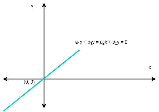
Graphical Representation

Suppose there are two lines

\begin{aligned} &a_1x + b_1y = 0\\\\ &a_2x + b_2y = 0 \end{aligned}

When two lines intersect at a single point there is only one unique solution. In the case of homogeneous linear equations the point of interaction is the origin $(x =y = 0)$ .

Figure 1 – Only Trivial Solution To Homogeneous System Of Linear Equations

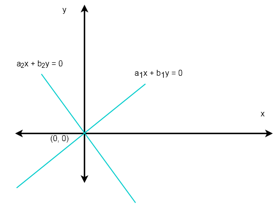
If the homogeneous system linear equations has $m$ equations with $n$ unknowns where $m \gt n$ then we can say that it is guaranteed to have a non-trivial solutions.

Figure 2 – Non-Trivial Solutions To Homogeneous System Of Linear Equations

To solve a system of linear equation we perform Gauss-Jordan elimination and the augmented matrix is reduced to echelon form or reduced row echelon form. We use the same elimination technique to reduce the homogeneous system of linear equations. For example, consider following homogeneous system of linear equations.

\begin{aligned} &x_2 + x_4 = 0\\\\ &x_1 - x_3 + x_4 = 0\\\\ &2x_3 - 2x_4 = 0 \end{aligned}

From the above homogeneous system of linear equations we obtained following augmented matrix.

\begin{aligned} A = \begin{bmatrix}2 & -1 & 0 & 1 & 0\\1 & 0 & -1 & 1 & 0\\0 & 0 & 2 & -2 & 0\end{bmatrix} \end{aligned}

Perform the Gauss-Jordan Elimination on the matrix $A$

\begin{aligned} &R3 = \frac{R3}{2} \end{aligned}

\begin{aligned} &A = \begin{bmatrix}2 & -1 & 0 & 1 & 0\\1 & 0 & -1 & 1 & 0\\0 & 0 & 1 & -1 & 0\end{bmatrix} \end{aligned}

\begin{aligned} R1 \longleftrightarrow R2 \end{aligned}

\begin{aligned} &A = \begin{bmatrix}1 & 0 & -1 & 1 & 0\\2 & -1 & 0 & 1 & 0\\0 & 0 & 1 & -1 & 0\end{bmatrix} \end{aligned}

\begin{aligned} R2 = R2 - 2R1 \end{aligned}

\begin{aligned} &A = \begin{bmatrix}1 & 0 & -1 & 1 & 0\\0 & -1 & 2 & -1 & 0\\0 & 0 & 1 & -1 & 0\end{bmatrix} \end{aligned}

The matrix $A$ is in echelon form and we obtained new homogeneous system of linear equations.

\begin{aligned} &x_1 - x_3 + x_4 = 0\\\\ & -x_2 + 2x_3 - x_4 = 0\\\\ &x_3 - x_4 = 0 \end{aligned}

The first variable in each equation is called basic variable and other variables are free variables.

Let basic variables be $b_n$ and free variables be $f_1, f_2, ...f_n$ for $n \in N$ .

\begin{aligned} b_n = \sum f_1 + f_2 ... f_n \end{aligned}

Using the above, the reduced form of homogeneous system of linear equation becomes

\begin{aligned} &x_1 = x_3 - x_4\\\\ &x_2 = 2x_3 - x_4\\\\ &x_3 = x_4\\\\ &x_4 = c \end{aligned}

Therefore, the general solution for the given homogeneous system of linear equation is

\begin{aligned} &x_1= x_3 - c\\\\ &x_2= 2x_3 - c\\\\ &x_3 = c\\\\ &x_4 = c \end{aligned}

We can make few conclusions based on the example above.

The echelon form of a homogeneous system of linear equations is also a homogeneous linear equations.
The non-trivial solution is possible, if m equations and n unknowns with m <= n and after the matrix A is reduced to echelon form with t non-zero rows obtained where t < n.

Relationship Between Non-Homogeneous System And Homogeneous System

There is a relationship between non-homogeneous system of linear equations and homogeneous systems which allows to obtain all solutions to non-homogeneous systems.

Let $A$ be a matrix of size $m \times n$ and $b$ be a column matrix of size $m \times 1$ such that $Ax = b$ is consistent with a solution $s_1$ Then every solution $s$ can be written as

s = s_1 + p

where p is solution to homogeneous system of linear equations $A.x = 0$ which means $A.p =0$ .

This kind of solution is obtained by linear translations about which you will learn in future articles.

post

Trace Of Matrix

Matrix has a special function called trace function. If $A$ is a square matrix then the sum of its main diagonal entry is called trace of matrix $A$ and is denoted by $tr(A)$ .

Let $A$ be a square matrix with size $n\times n$ , then

\begin{aligned} A = \begin{bmatrix}a_{11} & a_{12} & a_{13}\\a_{21} & a_{22} & a_{23}\\a_{31} & a_{32} & a_{33}\end{bmatrix} \end{aligned}

The trace of matrix is,

\begin{aligned} tr(A) = a_{11} + b_{22} + c_{33} \end{aligned}

Let is see few examples of traces of matrices.

Example #1

Let A be a square matrix of size $3 \times 3$

\begin{aligned} A = \begin{bmatrix}-1 & 4 & 2\\6 & 2 & 7\\5 & 1 & 8\end{bmatrix} \end{aligned}

The trace of the matrix A is,

\begin{aligned} &tr(A) = (-1) + 2 + 8 = 9\\\\ &tr(A) = 9 \end{aligned}

Example #2

Let B be a square matrix of size $4 \times 4$ .

\begin{aligned} B = \begin{bmatrix}6 & 1 & 1 & -2\\5 & 9 & -1 & 3\\0 & 1 & 7 & 2\\3 & 7 & 8 & 5\end{bmatrix} \end{aligned}

The trace of matrix B is,

\begin{aligned} &tr(B) = 6 + 9 + 7 + 5 = 27\\\\ &tr(B) = 27 \end{aligned}

If the matrix A is not a square matrix, then $tr(A)$ is not defined.

post

Matrix Transpose

The transpose of a matrix is denoted by $A^T$ is obtained by changing rows into columns or columns to rows of a matrix $A$ . If size of the matrix $A$ is $m \times n$ then the size of the transposed matrix $A^T$ is $n \times m$ .

Transpose Of A Matrix

The element in $i^{th}$ row and $j^{th}$ column of matrix $A$ becomes the $j^{th}$ row and $i^{th}$ column element in matrix $A^T$ .

\begin{aligned} &(A^T)_{ij} = (A)_{ji} \end{aligned}

Let $A$ be a matrix of size $m \times n$ .

\begin{aligned} A = \begin{bmatrix}a & b\\ c & d\\ e & f\end{bmatrix} \end{aligned}

Transpose of matrix $A$ .

\begin{aligned} A^T = \begin{bmatrix}a & c & e\\ b & d & f\end{bmatrix} \end{aligned}

Let us take element ‘c’ which is at 2nd row and 1st column of matrix $A$ ; after transpose operation on matrix $A$ , it is at the position of 1st row and 2nd column of matrix $A^T$ .

Similarly, the element ‘b’ is at the position of first row and second column of matrix $A$ , but after the transpose operation, its position changes to 2nd row and 1st column in matrix $A^T$ .

Example #1

Transpose the following matrix A.

\begin{aligned} A = \begin{bmatrix}3 & 1 & 5\\ 2 & 6 & 9\end{bmatrix} \end{aligned}

The transpose of matrix $A$ is

\begin{aligned} A^T = \begin{bmatrix}3 & 2\\ 1 & 6\\5 & 9\end{bmatrix} \end{aligned}

Example #2

Transpose the following matrix B.

\begin{aligned} &A = \begin{bmatrix}1 & 5\\ 7 & 6\\8 & 4\end{bmatrix} \end{aligned}

The transpose of matrix $A^T$ is

\begin{aligned} A^T = \begin{bmatrix}1 & 7 & 8\\ 5 & 6 & 4\end{bmatrix} \end{aligned}

Symmetric Matrix

When the transpose of the matrix is the original matrix itself, then it is called a Symmetric matrix. Suppose $A$ is a matrix of size $m \times n$ , then the transpose of matrix $A = A^T$ .

All the elements above the diagonal is a mirror image of elements below the diagonal elements. That is, $A = [a_{ij}]_{m \times n}$ is symmetric matrix if $(A)_{ij} = (A)_{ji}$ for all i and j.

\begin{aligned} A = \begin{bmatrix}a_{11} & p & q\\p & a_{22} & r\\q & r & a_{33}\end{bmatrix} \end{aligned}

The elements of $(A)<em>{ij} = (A)</em>{ji}$ . The transpose of such a matrix is,

\begin{aligned} A^T = \begin{bmatrix}a_{11} & p & q\\p & a_{22} & r\\q & r & a_{33}\end{bmatrix} \end{aligned}

Therefore,

\begin{aligned} A = A^T \end{aligned}

What Are The Properties Of A Transpose Of A Matrix ?

In this section, we shall discuss about the properties of a transpose of a matrix. There are 4 interesting properties of a transpose as listed below.

$(A^T)^T = A$ , where $A$ is a matrix of size $m \times n$ or $n \times n$ .
$(A + B)^T = A^T + B^T$ , where $A$ and $B$ are of same size, that is, $m \times n$ or $n \times n$ .
$(rA)^T = rA^T$ , where $A$ is matrix of size $m \times n$ or $n \times n$ and $r$ is a real number.
$(AB)^T = B^TA^T$ , where $A$ and $B$ are matrices of size $A_{m \times n}$ and $B_{n \times p}$ .

Let us verify each of the statement.

#1 : $(A^T)^T = A$

The transpose of a transpose of matrix $A$ is the original matrix $A$ .

\begin{aligned} Let \hspace{5px}A = \begin{bmatrix}2 & 3\\-1 & 5\end{bmatrix} \end{aligned}

Transpose of matrix $A$ .

\begin{aligned} A^T = \begin{bmatrix}2 & -1\\3 & 5\end{bmatrix} \end{aligned}

Transpose of $A^T$ .

\begin{aligned} (A^T)^T = \begin{bmatrix}2 & 3\\-1 & 5\end{bmatrix} \end{aligned}

From the results above, it is clear that $(A^T)^T = A$ where $A$ is a matrix of size $m \times n$ or $n \times n$ .

#2 : $(A + B)^T = A^T + B^T$

The transpose of sum of two matrices $A$ and $B$ of same size $m \times n$ or $n \times n$ is equal to sum of transpose of matrices $A$ and $B$ .

Let $A$ and $B$ be two matrices of same size. Then

\begin{aligned} &A = \begin{bmatrix}1 & 5\\-2 & 3\end{bmatrix} B = \begin{bmatrix}2 & 1\\5 & -1\end{bmatrix}\\\\ &(A + B) = \begin{bmatrix}3 & 6\\3 & 2\end{bmatrix} \end{aligned}

Transpose of matrix $(A + B)^T$ .

\begin{aligned} (A + B)^T = \begin{bmatrix}3 & 3\\6 & 2\end{bmatrix} \end{aligned}

Now, we shall take transpose of matrix $A$ and matrix $B$ and add them together to obtain $A^T + B^T$ .

\begin{aligned} A = \begin{bmatrix}1 & 5\\-2 & 3\end{bmatrix} B = \begin{bmatrix}2 & 1\\5 & -1\end{bmatrix} \end{aligned}

Transpose of A.

\begin{aligned} A^T = \begin{bmatrix}1 & -2\\5 & 3\end{bmatrix} \end{aligned}

Transpose of B.

\begin{aligned} B^T = \begin{bmatrix}2 & 5\\1 & -1\end{bmatrix} \end{aligned}

Sum of $A^T$ and $B^T$ .

\begin{aligned} A^T + B^T = \begin{bmatrix}3 & 3\\6 & 2\end{bmatrix} \end{aligned}

#3 : $(rA)^T = rA^T$

A transpose of the product of matrix $A$ with scalar $r$ is equal to the product of scalar $r$ and transpose of matrix $A$ where size of the matrix $A$ is $m \times n$ or $n \times n$ and $r$ is a real number.

\begin{aligned} &Let \hspace{5px} A = \begin{bmatrix}2 & 3\\1 & 7\end{bmatrix} \hspace{4px} and \hspace{5px} r = 2\\\\ &(rA) = \begin{bmatrix}4 & 6\\2 & 14\end{bmatrix} \end{aligned}

Transpose of $rA$ ,

\begin{aligned} (rA)^T = \begin{bmatrix}4 & 2\\6 & 14\end{bmatrix} \end{aligned}

Similarly, let us take transpose of $A$ .

\begin{aligned} A^T = \begin{bmatrix}2 & 1\\3 & 7\end{bmatrix} \end{aligned}

The product $rA^T$ is,

\begin{aligned} rA^T = \begin{bmatrix}4 & 2\\6 & 14\end{bmatrix} \end{aligned}

Therefore, $(rA)^T = rA^T$ .

The output of both the products are equal and the property $(rA)^T = rA^T$ is true for all matrices.

#4 : $(AB)^T = B^TA^T$

The transpose of product of two defined ( $A_{m \times n}$ and $B_{n \times p}$ ) matrices $A$ and $B$ is equal to the product of transpose of matrix $B$ and transpose of matrix $A$ . Let us verify this claim with the help of an example.

\begin{aligned} &Let \hspace{5px}A = \begin{bmatrix}1 & 5\\2 & 1\end{bmatrix} \hspace{5px} and \hspace{5px} B = \begin{bmatrix}3 & -1\\2 & 3\end{bmatrix}\\\\ &AB = \begin{bmatrix}3 + 10 & -1 + 15\\6 + 2 & -2 + 3\end{bmatrix}= \begin{bmatrix}13 & 14\\8 & 1\end{bmatrix} \end{aligned}

Transpose of $AB$ .

\begin{aligned} (AB)^T = \begin{bmatrix}13 & 8\\14 & 1\end{bmatrix} \end{aligned}

Similarly, the transpose of matrix $B$ and matrix $A$ is,

\begin{aligned} &B^T = \begin{bmatrix}3 & 2\\-1 & 3\end{bmatrix} \hspace{5px} and \hspace{5px} A^T = \begin{bmatrix}1 & 2\\5 & 1\end{bmatrix}\\\\ &B^TA^T = \begin{bmatrix}3 + 10 & 6 + 2\\-1 + 15 & -2 + 3\end{bmatrix}\\\\ &B^TA^T = \begin{bmatrix}13 & 8\\14 & 1\end{bmatrix}\\\\ &Therefore, \hspace{5px}(AB)^T = B^TA^T \end{aligned}

Once again, the product of both sides of the equation of the property $(AB)^T = B^TA^T$ holds true. The property is valid.

In the next, post we will discuss more about symmetric and skew-symmetric matrices.

post

Matrix Multiplication

The multiplication of matrices means rows of matrix $A$ is multiplied to columns of $B$ to obtain a third matrix $C$ . We also evaluate the matrix multiplication with respect to fundamental properties of mathematics such as commutative, associative property, identity property.

Conditions for Matrix Multiplication

If $A_{m \times n}$ and $B_{n \times p}$ are two matrices with sizes $m \times n$ and $n \times p$ respectively. The following conditions apply to matrix multiplication,

Row or column of matrix $A$ must be equal to column or row of matrix $B$ .
Multiplying matrix $A$ to matrix $B$ is not same as multiplying matrix $B$ i.e., $AB \neq BA$ .
If condition 2 and 3 are true, then we can multiply 2 or more matrices.

Matrix Multiplication

Let $A_{1 \times n}$ and $B_{n \times 1}$ be two matrices with elements. Then the matrix multiplication can be done as follows.

\begin{aligned} &A = \begin{bmatrix}a_{11} & a_{12}& . . . & a_{1n}\end{bmatrix} B = \begin{bmatrix}b_{11} \\ b_{21} \\ : \\ b_{n1}\end{bmatrix}\\\\ &C_{1 \times 1} = A . B = \begin{bmatrix}a_{11}b_{11} + a_{12}b_{21} + ... + a_{1n}b_{n1}\end{bmatrix} \end{aligned}

In the above example, $A$ has size $m \times n$ where $m = 1$ and $B$ has size $n \times p$ where the resultant matrix $C$ has size of $m \times p$ which is $1 \times 1$ .

Now, we consider the second case, where we multiply $B$ to $A$ .

\begin{aligned} &B = \begin{bmatrix}b_{11} \\ b_{21} \\ : \\ b_{n1}\end{bmatrix} A = \begin{bmatrix}a_{11} & a_{12}& . . . & a_{1n}\end{bmatrix}\\\\ &C_{n \times n} = A . B = \begin{bmatrix}b_{11}a_{11} & b_{11}a_{12} & ... & b_{11}a_{1n}\\ b_{21}a_{11} & b_{21}a_{11} & ... & b_{21}a_{1n}\\ : & : & : & :\\ b_{n1}a_{11} & b_{n1}a_{12} & ... & b_{n1}a_{1n}\end{bmatrix} \end{aligned}

Matrix Multiplication Examples

In this section, we will show you few examples with different kinds of matrices.

Example #1

\begin{aligned} &// \hspace{5px} Multiplying \hspace{5px} Square \hspace{5px}Matrix\\\\ &A_{2 \times 2} = \begin{bmatrix}2 & 3 \\ 1 & 7\end{bmatrix} B_{2 \times 2} = \begin{bmatrix}2 & 3\\ 1 & 1\end{bmatrix}\\\\ &AB = \begin{bmatrix}(2 * 2)+ (3 * 1) & (2 * 3)+ (3 * 1)\\ (1 * 2) + (7 * 1) & (1 * 3) + ( 7 * 1)\end{bmatrix}\\\\ &AB = \begin{bmatrix}(4)+ (3) & (6)+ (3)\\ (2) + (7) & (3) + (7)\end{bmatrix}\\\\ &AB_{2 \times 2} = \begin{bmatrix}7 & 9\\ 9 & 10\end{bmatrix} \end{aligned}

The size of matrix $A$ is $m \times n$ where $m = n$ and size of matrix $B$ is also $n \times p$ where $n = p$ . Therefore, resultant matrix after multiplication has a size of $m \times p$ where $m = p$ . In other words, $A_{2 \times 2} \times B_{2 \times 2} = C_{2 \times 2}$ .

Example #2

\begin{aligned} &A_{2 \times 3} = \begin{bmatrix}4 & -1 & 1\\ 4 & 1 & -2\end{bmatrix} B_{3 \times 2} = \begin{bmatrix}2 & -2\\ 1 & -2 \\ 5 & 2\end{bmatrix}\\\\ &AB = \begin{bmatrix}(4 * 2)+ (-1 * 1) + (1 * 5) & (4 * -2)+ (-1 * -2) + (1 * 2)\\ (4 * 2) + (1 * 1) + (-2 * 5) & (4 * -2) + ( 1 * -2) + (-2 * 2)\end{bmatrix}\\\\ &AB = \begin{bmatrix}(8)+ (-1) + (5) & (-8)+ (2) + (2)\\ (8) + (1) + (-10) & (-8) + (-2) + (-4)\end{bmatrix}\\\\ &AB = \begin{bmatrix}12 & -4\\ -1 & -14\end{bmatrix} \end{aligned}

The size of the matrix $A$ is $m \times n$ where $m = 2$ and the size of the matrix $B$ is $n \times p$ where $p = 2$ . Therefore, the resultant matrix $AB$ has a size of $m \times p$ which is $2 \times 2$ .

Example #3

\begin{aligned} &A_{3 \times 2} = \begin{bmatrix}1 & 1 \\ 3 & 5 \\ 2 & 3\end{bmatrix} B_{2 \times 3} = \begin{bmatrix}3 & 1 & 0\\ 7 & 4 & 1 \end{bmatrix}\\\\ &AB = \begin{bmatrix}(1 * 3)+ (1 * 7) & (1 * 1) + (1 * 4) & (1 * 0) + (1 * 1)\\ (3 * 3)+ (5 * 7) & (3 * 1) + (5 * 4) & (3 * 0) + (5 * 1)\\ (2 * 3)+ (3 * 7) & (2 * 1) + (3 * 4) & (2 * 0) + (3 * 1)\\\end{bmatrix}\\\\ &AB = \begin{bmatrix}(3)+ (7) & (1) + (4) & (0) + (1)\\ (9)+ (35) & (3) + (20) & (0) + (5)\\ (6)+ (21) & (2) + (12) & (0) + (3)\\\end{bmatrix}\\\\ &AB = \begin{bmatrix}10 & 4 & 1\\ 44 & 23 & 5\\ 27 & 14 & 3\end{bmatrix} \end{aligned}

The matrix $A$ has a size of $m \times n$ where $m = 3$ and matrix $B$ has a size of $n \times p$ where $p = 3$ . The size of resultant matrix $AB$ is $m \times p$ which is $3 \times 3$ .

Properties of Matrix Multiplication

Since, matrix operation is mathematical operations, therefore, matrix multiplication must preserve all or some of the properties with respect to multiplication operator.

Commutative Law

Suppose we multiply two matrix $A$ and $B$ ,

\begin{aligned} &A = \begin{bmatrix}2 & 2\\ 3 & 1\end{bmatrix} B = \begin{bmatrix}1 & 2\\ 5 & 2\end{bmatrix}\\\\ &AB = \begin{bmatrix}12 & 8\\ 8 & 8\end{bmatrix}\\\\ &Similarly, \\\\ &B = \begin{bmatrix}1 & 2\\ 5 & 2\end{bmatrix} A = \begin{bmatrix}2 & 2\\ 3 & 1\end{bmatrix}\\\\ &BA = AB = \begin{bmatrix}8 & 4\\ 16 & 12\end{bmatrix}\\\\ &AB \neq BA \end{aligned}

From the example above, it is clear that the product of $AB$ is not equal to the product of $BA$ . Hence, the commutative law does not work in the case of matrix multiplication.

Associative Law of Matrix Multiplication

The associative law in matrix multiplication involves more than two matrices in following ways.

Let A, B, and C be three matrices that meet the conditions of matrix multiplication.Then,

\begin{aligned} A * ( B * C ) = (A * B) * C \end{aligned}

We can test the above property with the help of an example. Let $A, B$ and $C$ be 3 square matrices of size $2 \times 2$ .

\begin{aligned} &A = \begin{bmatrix}1 & 2\\3 & 4\end{bmatrix} B = \begin{bmatrix}2 & 3\\4 & 5\end{bmatrix} C = \begin{bmatrix}3 & 2\\1 & 1\end{bmatrix}\\\\ &BC = \begin{bmatrix}9 & 7\\17 & 13\end{bmatrix}\\\\ &A * (BC) = \begin{bmatrix}43 & 33\\95 & 73\end{bmatrix}\\\\ &Similarly, \\\\ &AB = \begin{bmatrix}10 & 13\\22 & 29\end{bmatrix}\\\\ &(AB) * C = \begin{bmatrix}43 & 33\\95 & 73\end{bmatrix}\\\\ &Therefore, \\\\ &A * (B * C) = (A * B) * C \end{aligned}

The above example, both side of the equation gives same results. Thus, the associative law is true for matrix multiplication.

Identity Law

In mathematics, an identity element is a value when added element ‘a’ will give ‘a’ itself. We know that identity of addition is 0.

\begin{aligned} &a + 0 = a\\\\ &For \hspace{5px}multiplication,\\\\ &a * 1 = 1 \end{aligned}

Since, 1 is the identity element of multiplication, we need a matrix with main diagonals as 1s, such a matrix is called an identity matrix or unit matrix denoted by $I_{n}$ where $n$ is the size $n \times n$ . Therefore, identity matrix is a square matrix.

Let A be a square matrix of size 2 x 2 and I be identity matrix of size 2 x 2. Then,

\begin{aligned} &A = \begin{bmatrix}2 & 4\\4 & 6\end{bmatrix} I_{2} = \begin{bmatrix} 1 & 0\\0 & 1\end{bmatrix}\\\\ &A.I_{2} = \begin{bmatrix}2 + 0 & 0 + 4\\4 + 0 & 0 + 6\end{bmatrix}\\\\ &A.I_{2} = \begin{bmatrix}2 & 4\\4 & 6\end{bmatrix} \end{aligned}

The unit matrix when multiplied with matrix $A$ gives the same matrix $A$ as result. Therefore, identity law is true for matrix multiplication.

Commutative Property For Identity Law

We mentioned earlier that the commutative property does not apply for matrix multiplication. However, in the case of multiplying a matrix $A$ with an identity matrix $I_{n}$ , the commutative property is true.

For example, let us take previous example where we found following results.

\begin{aligned} A.I_{2} = \begin{bmatrix}2 & 4\\4 & 6\end{bmatrix} \end{aligned}

We must find $I_{n}A$ to verify our claim that the commutative law does work when multiplied with an identity matrix.

Let A be a square matrix of size 2 x 2 and I be identity matrix of size 2 x 2. Then

\begin{aligned} &I_{2} = \begin{bmatrix} 1 & 0\\0 & 1\end{bmatrix} A = \begin{bmatrix}2 & 4\\4 & 6\end{bmatrix}\\\\ &I_{2}. A = \begin{bmatrix}2 + 0 & 4 + 0\\0 + 4 & 0 + 6\end{bmatrix}\\\\ &A.I_{2} = \begin{bmatrix}2 & 4\\4 & 6\end{bmatrix} \end{aligned}

Clearly, commutative law is true in the case of matrix multiplication if one of the matrix is identity matrix. You can try to perform the multiplication with more than two matrices. Therefore, $A.I_{n} = I_{n}.A = A$ .

In the next post, we will discuss about taking transpose of a matrix.

post

Matrix Subtraction

In the previous post, you have learned about matrix addition and its mathematical properties. The matrix subtraction is also mathematical operation on two matrices where elements of right hand matrix is subtract from elements of matrix on the left hand. The result is stored in a separate third matrix.

Condition To Subtract Matrices

Similar to matrix addition, there are few conditions for matrix subtraction. The minuend matrix should be on the left hand side and subtrahend matrix on the right The result of the subtraction must be stored in a difference matrix. The size of all three matrices must be same.

\begin{aligned} &\hspace{5px}A - B = C\\\\ &=\begin{bmatrix} a_{11} & a_{12} & a_{13}\\a_{21} & a_{22} & a_{23}\\a_{31} & a_{32} & a_{33}\end{bmatrix} - \begin{bmatrix} b_{11} & b_{12} & b_{13}\\b_{21} & b_{22} & b_{23}\\b_{31} & b_{32} & b_{33}\end{bmatrix}\\\\ & =\begin{bmatrix} a_{11}- b_{11} & a_{12}- b_{12} & a_{13}- b_{13}\\a_{21}-b_{21} & a_{22}-b_{22} & a_{23}- b_{23}\\a_{31} - b_{31}& a_{32} - b_{32} & a_{33} - b_{33}\end{bmatrix}\\\\ &C =\begin{bmatrix} c_{11} & c_{12} & c_{13}\\c_{21} & c_{22} & c_{23}\\c_{31} & c_{32} & c_{33}\end{bmatrix} \end{aligned}

The matrix $A$ is minuend and matrix $B$ is subtrahend. The difference is stored in the matrix $C$.

Mathematical Properties of Matrix Subtraction

The properties of matrix addition such as commutative, associative , scalar multiplication, also applies to subtraction, in other words, the elements of both matrix are performing addition, but one or more elements happen to be negative number.

For example, another way to look at the matrix subtraction is as follows where $A$ and $B$ are two matrices.

\begin{aligned} A - B = A + (-1 * B ) = C \end{aligned}

The above equation will yield same results.

Example

In this example, we will subtract matrix $B$ from matrix $A$ and keep the difference in matrix $C$.

\begin{aligned} &A - B = C\\\\ &=\begin{bmatrix} 5 & 4 & 3\\1 & 2 & 3\\9 & 8 & 7\end{bmatrix} - \begin{bmatrix} 2 & 1 & 0\\1 & 1 & 1\\2 & 4 & 5\end{bmatrix}\\\\ &=\begin{bmatrix} 5 - 2 & 4 - 1 & 3 - 0\\1 - 1 & 2 - 1 & 3 - 1\\9 - 2 & 8 - 4 & 7 - 5\end{bmatrix}\\\\ &C =\begin{bmatrix} 3 & 3 & 3\\0 & 1 & 2\\7 & 4 & 2\end{bmatrix} \end{aligned}

Though the above example shows positive elements, its not always true and one must careful while subtracting from a negative numbers as the sign must change.

post

Matrix Addition

Previous article, you learned that matrix are two dimensional representation of data other than augmented matrix from a system of linear equations. Matrix operations such as addition is possible because you can add two matrices $latex A&s=1$ and $latex B&s=1$ by simply adding their corresponding elements which will give a thrid matrix as a result.

Condition To Add Two Matrices

You can add a matrix like ordinary numbers simply by adding each corresponding elements of two matrices. This is only possible if size of both matrices are same.

Also, the order of matrix addition is not important because addition has commutative property.

Let $A$ and $B$ be two matrices of same size.

\begin{aligned} &A_{2 \times 3} = \begin{bmatrix} a_{11} & a_{12} & a_{13}\\a_{21} & a_{22} & a_{23}\end{bmatrix}_{2 \times 3}\\\\ &B_{2 \times 3} = \begin{bmatrix} b_{11} & b_{12} & b_{13}\\b_{21} & b_{22} & b_{23}\end{bmatrix}_{2 \times 3} \end{aligned}

Both matrices of same size and the order of addition does not matter, then

\begin{aligned} &C_{2 \times 3} = A_{2 \times 3} + B_{2 \times 3} = B_{2 \times 3} + A_{2 \times 3}\\\\ &C_{2 \times 3} = \begin{bmatrix} a_{11} + b_{11} & a_{12} + b_{12} & a_{13} + b_{13}\\a_{2 \times 3} + b_{21} & a_{22} + b_{22} & a_{23} + b_{23}\end{bmatrix}\\\\ &C_{2 \times 3} = \begin{bmatrix} c_{11} & c_{12} & c_{13}\\c_{21} & c_{22} & c_{23}\end{bmatrix} \end{aligned}

Properties of Matrix Addition

The addition operation has certain fundamental properties that applies to all real numbers. Since, matrix addition is also a common addition, these fundamental mathematical properties applies to them as well.

Commutative Property

If A and B are two independent matrices of same size, then

\begin{aligned} &A + B = B + A \end{aligned}

Example

\begin{aligned} &A = \begin{bmatrix} 1 & 2 & 3\\6 & 5 & 4\end{bmatrix} \hspace{3ex} B = \begin{bmatrix} 2 & 1 & 5\\1 & 1 & 0\end{bmatrix} \end{aligned}

\begin{aligned} C = A + B = \begin{bmatrix} 3 & 3 & 8\\7 & 6 & 4\end{bmatrix} = B + A \end{aligned}

Associative Property

If A, B and C are three matrices of same size then,

\begin{aligned} (A + B)+ C = A + (B + C) \end{aligned}

Example

\begin{aligned} A = \begin{bmatrix} 1 & 2 & 3\\6 & 5 & 4\end{bmatrix} \hspace{3ex} B = \begin{bmatrix} 2 & 1 & 5\\1 & 1 & 0\end{bmatrix} \hspace{3ex} C = \begin{bmatrix} 1 & 1 & 1\\1 & 2 & 1\end{bmatrix} \end{aligned}

\begin{aligned} &(A + B) + C = \begin{bmatrix} 3 & 3 & 8\\7 & 6 & 4\end{bmatrix} + \begin{bmatrix} 1 & 1 & 1\\1 & 2 & 1\end{bmatrix}\\\\ &(A + B) + C = \begin{bmatrix} 4 & 4 & 9\\8 & 8 & 5\end{bmatrix} \end{aligned}

Similarly,

\begin{aligned} &A + (B + C) = \begin{bmatrix} 1 & 2 & 3\\6 & 5 & 4\end{bmatrix} + \begin{bmatrix} 3 & 2 & 6\\2 & 3 & 1\end{bmatrix}\\\\ &A + (B + C) = \begin{bmatrix} 4 & 4 & 9\\8 & 8 & 5\end{bmatrix} \end{aligned}

Identity Property

The identity element for addition (+) is $0$. You add $0$ to element $a + 0 = a$. The result is always $a$. Therefore, if we add matrix A to a zero matrix, the result is A matrix itself.

\begin{aligned} A + O = A \end{aligned}

Example

\begin{aligned} &A = \begin{bmatrix} 1 & 2 & 3\\6 & 5 & 4\end{bmatrix} \hspace{3ex} O = \begin{bmatrix} 0 & 0 & 0\\0 & 0 & 0\end{bmatrix}\\\\ &A + O = \begin{bmatrix} 1 & 2 & 3\\6 & 5 & 4\end{bmatrix} \end{aligned}

There are other interesting properties of matrix addition which we discuss in future posts.

post

Matrix Operations

In this section, you will learn common mathematical operations performed on matrices. These operations range from common arithmetic operations such as addition, subtraction, multiplication to transpose matrices.

Before we proceed to learn about matrix operations, you should learn common matrix notations and terminologies used in this section.

Common Matrix Notations

An augmented matrix is derived from the system of linear equations, but there are other areas where a matrix appear as two dimensional data set with rows and columns. In general,

“A matrix is rectangular arrays of numbers called entries of the matrix”

Example

\begin{aligned} A = \begin{bmatrix} 1 & 2 & 3\\4 & 5 & 6\\7 & 8 & 9\end{bmatrix} B = \begin{bmatrix} a_{11} & a_{12} & a_{13}\\a_{21} & a_{22} & a_{23}\\a_{31} & a_{32} & a_{33}\end{bmatrix} \end{aligned}

The matrix itself is denoted by a capital letter such as $A$ or $B$ . The entries of matrices are real numbers that are denoted with lowercase letters such as $a, b, c$ etc. The subscript to the entry element denotes the position of the element within the matrix. For example,

If A is the matrix, then

\begin{aligned} (A)_{ij} = a_{ij} \end{aligned}

where i is row number and j is the column number.

Size of the Matrix

The size of the matrix is denoted in terms of its rows and columns. Given a matrix, the size is $m \times n$ where $m$ is rows and $n$ is columns. You can use any letters to represent rows and columns, however, common practice is to use $m$ and $n$ .

\begin{aligned} C_{2 \times 3} = \begin{bmatrix} a_{11} & a_{12} & a_{13}\\a_{21} & a_{22} & a_{23}\end{bmatrix}_{2 \times 3} \end{aligned}

The shortcut notation to represent a matrix is $[a_{ij}]_{m \times n}$ or $[a_{ij}]$ .

A matrix of size $1 \times n$ is a row matrix and $m \times 1$ is a column matrix which can be denoted using bold lowercase letters.

\begin{aligned} &\textbf{a} = \begin{bmatrix} a_{11} & a_{12} & ... & a_{1n}\end{bmatrix}\\\\ &\textbf{c} = \begin{bmatrix} c_{11} \\ c_{12} \\ : \\ : \\ c_{m1}\end{bmatrix} \end{aligned}

Equality Of Matrix

How do we know if two matrices are equal?

Two matrices, $A$ and $B$ are equal i.e, $A = B$ if and only if $a_{ij} = b_{ij}$ .

Two matrices are equal if and only if their size are equal and all entries are equal.

Example

Let their be four matrices – $A, B, C, D$ .

\begin{aligned} &A = \begin{bmatrix} 1 & 3\\ 2 & 5\end{bmatrix}_{2 \times 2}\\\\ &B = \begin{bmatrix} 4 & 1\\ -1 & 6\\ 3 & -1\end{bmatrix}_{3 \times 2}\\\\ &C = \begin{bmatrix} 1 & 3\\ 2 & 5\end{bmatrix}_{2 \times 2}\\\\ &D = \begin{bmatrix} 0 & 3\\ 7 & 5\end{bmatrix}_{2 \times 2} \end{aligned}

Lets compare matrix A with other matrices.

$A \neq B$ because the size and elements does not match at all.

$A = C$ because the size and elements does match perfectly.

$A \neq D$ because the size match but the elements $a_{ij} \neq d_{ij}$ for some corresponding elements.

Common Matrix Operations

There are many elementary row operation about which you learned in the previous sections. However, we can perform some basic mathematical operations on elements of matrix as well. There are

Matrix Addition
Matrix Subtraction
Matrix Multiplication
Scalar Multiplication With Matrix
Transpose Matrix
Trace Of Matrix

The above are some common matrix operations you will find through linear algebra course. There are some advanced and complex operations about which we discuss in later part of the linear algebra tutorial.

post

Gaussian Elimination

Gaussian elimination is a technique to change the augmented matrix into a row echelon form.There are many echelon forms, but subsequently, we must find the reduced row echelon form. The reduced row echelon form can can be achieved through another technique called the Gauss-Jordan elimination technique.

Augmented Matrix To Row Echelon Form

Given an augmented matrix that represents a system of linear equations with n equations and m variables. We want to reduce the matrix to a simple form called the echelon form and solve the unknowns.

\begin{aligned} &5x + y + z = 10\\ &2x + y - 3z = -5\\ &x - 2y + 2z = 3 \end{aligned}

These are the steps to achieve the row echelon form.

Begin with column 1
Obtain leading 1 for each row and
Change 0 below all leading 1s.

Example

In this example we will convert the following augmented matrix into a row echelon form by series of row operations.

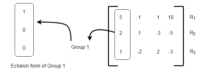
Figure 1 – Change the group 1 which is column 1 to echelon form by row operation.

Step 1

The augmented matrix first row starts with a leading 1 and all other entries in the first column are zeros. If the first row starts with a 0 , then do row exchange with second or third row and bring a non-zero value.

To obtain leading 1 in the first row do following row operation.

\begin{aligned} &R_{1} = \frac{R_{1}}{5} \end{aligned}

Our resultant matrix is as follows.

\begin{aligned} \begin{bmatrix} 1 & \frac{1}{5} & \frac{1}{5} & 2\\2 & 1 & -3 & -5\\1 & -2 & 2 & 3\end{bmatrix} \end{aligned}

Step 2

Perform following row operations to make rest of the entries 0 in the first column under leading 1.

\begin{aligned} &2R_{1}\\ &R_{3} =& R_{3} - R_{1} \end{aligned}

Now, our matrix look like the following.

\begin{aligned} \begin{bmatrix} 1 & \frac{1}{5} & \frac{1}{5} & 2\\0 & \frac{3}{5} & \frac{-17}{5} & -9\\0 & \frac{-11}{5} & \frac{9}{5} & 1\end{bmatrix} \end{aligned}

We must repeat the same steps for Group 2.

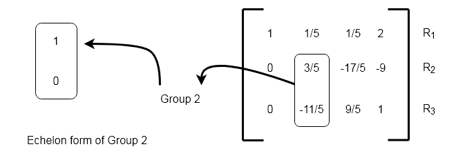
Figure 2 – Change Group 2 into row echelon form by performing row operations.

Step 3

In the group 2 which is column 2 , first change the value to leading 1.

\begin{aligned} &R_{2} = R_{2} * 5\\ &R_{2} = \frac{R_{2}}{3} \end{aligned}

The result of the row operation is given below.

\begin{aligned} \begin{bmatrix} 1 & \frac{1}{5} & \frac{1}{5} & 2\\0 & 1 & \frac{-17}{3} & -15\\0 & \frac{-11}{5} & \frac{9}{5} & 1\end{bmatrix} \end{aligned}

Step 4

All entries below leading 1 in second row must be changed to 0. Therefore, perform following row operations.

\begin{aligned} R_{3} = R_{3} + \frac{11}{5}R_{2} \end{aligned}

The result is as follows. The second row leading 1 has a 0 below it in the third row.

\begin{aligned} \begin{bmatrix} 1 & \frac{1}{5} & \frac{1}{5} & 2\\0 & 1 & \frac{-17}{3} & -15\\0 & 0 & \frac{-32}{3} & -32\end{bmatrix} \end{aligned}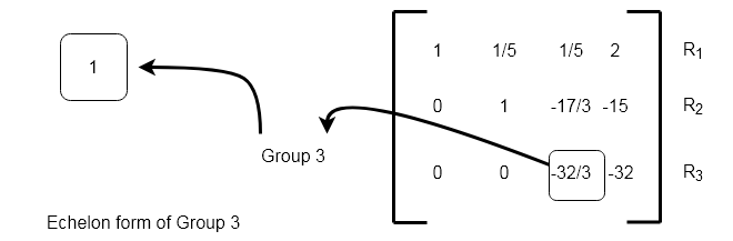

Figure 3 – Group 3 of the augmented matrix is only leading 1 of row 3

Step 5

Now, we must find the leading 1 for row 3. Do the following row operations on

\begin{aligned} &R_{3} = \frac{R_{3}}{-32}\\ &R_{3} = R_{3} * -3 \end{aligned}

The augmented matrix is in row echelon form and it is easy to find a solution to the matrix.

\begin{aligned} \begin{bmatrix} 1 & \frac{1}{5} & \frac{1}{5} & 2\\0 & 1 & \frac{-17}{3} & -15\\0 & 0 & 1 & 3\end{bmatrix} \end{aligned}

Back Substitution

The echelon form gives us the following simplified system of linear equations.

\begin{aligned} &x + \frac{y}{5} + \frac{z}{5} = 2\\ &y + \frac{-17}{3} = -15\\ &z = 3 \end{aligned}

Using value of z = 3$ and substituting in other equations,we get

\begin{aligned} &x + \frac{2}{5} + \frac{3}{5} = 2\\\\ &x = 2 - \frac{2}{5} - \frac{3}{5}\\\\ &x = \frac{10 - 2 - 3}{5}\\\\ &x = 1\\\\ &y - 17 = -15\\\\ &y = 17-15 = 2\\\\ &z = 3 \end{aligned}

Therefore, the solution to the equation is $x = 1, y =2, z = 3$.

post