Linear Algebra Archives - Page 3 of 3

Row Echelon Form

Previously, you learned about deriving an augmented matrix from a system of linear equations. You have also learned about reducing the augmented matrix into a simpler equivalent matrix that is easy to solve through series of row operations on the matrix. This kind of matrix form is known as the row echelon form of matrix.

Our goal for performing row operations on the matrix is to obtain the row echelon form or a reduced row echelon form from which deriving a solution to the system of linear equation is easy.

What is a Row Echelon Form of Matrix ?

The form of matrix that has following properties is said to be in row echelon form.

Rows with all 0s are pushed to the bottom of the matrix.
A row with first non-zero value as 1 is called leading 1.
The leading 1 in the lower row is to the farthest right than the leading 1 at row above it.
All other entries in the row except the last column as zero.

We now discuss each of the above points to explain the row echelon form.

Row with all zeros are pushed to the bottom

Suppose we are given a system of linear equations as follows.

\begin{aligned} &0x + 0y + 0z = 0\\ &2x + y + 2z = 10\\ &0x + 0y + 0z = 0\\ &x - 2y + z = 2 \end{aligned}

The augmented matrix that we derived is given below.

\begin{aligned} &A = \begin{bmatrix}0 & 0 & 0 & 0 \\2 & 1 & 2 & 10 \\0 & 0 & 0 & 0 \\1 & -2 & 1 & 2\end{bmatrix} \end{aligned}

Since, row that only zero does not give any proper solution to the system of equation it is of no use and pushed to the bottom of the matrix or eliminated subsequently.

\begin{aligned} &A = \begin{bmatrix}2 & 1 & 2 & 10 \\1 & -2 & 1 & 2\\0 & 0 & 0 & 0 \\0 & 0 & 0 & 0 \end{bmatrix} \end{aligned}

First non-zero value must be a 1

The first non-zero value of each row in echelon form must be a 1 called the leading 1. Consider following example,

\begin{aligned} &A = \begin{bmatrix}0 & 1 & 0 & 2 \\1 & 0 & 0 & 1\\0 & 0 & 1 & 3 \end{bmatrix} \end{aligned}

In the matrix above first non-zero element is a 1. Such a form is possible by a series of row operations on the original augmented matrix.

Leading 1 of lower row is to the farthest right than the row above

If you look at the previous, the matrix is still not in the echelon form because middle row has leading to the left than the leading 1 of the first row.

Figure 1 – The leading 1 of both row is not in correct order. A row exchange can solve the problem.

The leading 1 of the top row is to the right of the leading 1 of the the bottom row. To solve the problem, we do a row exchange between first and the second row. The result is in a row echelon form.

\begin{aligned} &A = \begin{bmatrix}1 & 0 & 0 & 1 \\0 & 1 & 0 & 2 \\0 & 0 & 1 & 3 \end{bmatrix} \end{aligned}

All other entries must be zero except the last column

Only if the other entries are zero, we could use back substitution for obtaining a solution to the matrix. The last column is not zero because it is part of the solution and we obtain the value of unknown from it. We will discuss about back substitution when we discuss about Gauss-Jordan elimination method for finding solution to the system of linear equations.

Difference Between Row Echelon Form and Reduced Row Echelon Form

In the row echelon form, the lower triangular matrix below the leading 1 is zero, whereas reduced row echelon form has both upper triangular and lower triangular values as zero with leading 1.

Row Echelon Example

\begin{aligned} A = \begin{bmatrix}1 & 0 & 3 & 1 \\0 & 1 & 5 & 2 \\0 & 0 & 1 & 3 \end{bmatrix} \end{aligned}

Reduced Row Echelon Form Example

\begin{aligned} A = \begin{bmatrix}1 & 0 & 0 & 1 \\0 & 1 & 0 & 2 \\0 & 0 & 1 & 3 \end{bmatrix} \end{aligned}

In a system of equations, there can be more than one row echelon form, however, there is only one reduced row echelon form of the matrix.

post

Elementary Row Operations

Earlier we learnt that we can solve for unknown variables by substituting arbitrary values for the equation. You can $a_{1}x_{1} + a_{2}x_{2} = b_{1}$ by solving for $x$ or $y$ one at a time.

Now, a system of equations have $m$ equations which we change into a new system having same solution set but simplified and easy to solve. This is achieved by performing row operations on the augmented matrix.

Row Operations

A row is a linear equation with $n$ unknown variables. You can perform following operations on any row in a system of equations.

Multiply a row with a scalar i.e., non-zero constant.
Add one row to another row. You are adding matching terms from one row to another.
Interchange two rows

Multiply A Row With A Non-Zero Scalar

\begin{aligned} &A = \begin{bmatrix}1 & 3 & 8 \\ 2 & 1 & 1 \\ 7 & 4 & 1\end{bmatrix}\\\\ &Now, row 1 ( R_{1} ) \hspace{5px} is \hspace{5px}\begin{bmatrix}1 & 3 & 8\end{bmatrix} which \hspace{5px}we \hspace{5px}multiply \hspace{5px}by \hspace{5px}2.\\\\ &R_{1} \times 2 = \begin{bmatrix}1 & 3 & 8\end{bmatrix} \times 2\\\\ &A = \begin{bmatrix}2 & 6 & 16 \\ 2 & 1 & 1 \\ 7 & 4 & 1\end{bmatrix} \end{aligned}

Adding One Row To Another Row

\begin{aligned} &A = \begin{bmatrix}1 & 3 & 8 \\ 2 & 1 & 1 \\ 7 & 4 & 1\end{bmatrix}\\\\ &Row 1 \hspace{5px}is \hspace{5px} \begin{bmatrix}1 & 3 & 8\end{bmatrix}\\\\ &Row 2 \hspace{5px}is \hspace{5px} \begin{bmatrix}2 & 1 & 1\end{bmatrix}\\\\ &Therefore,\hspace{5px} we \hspace{5px}can \hspace{5px} add \hspace{5px}row 1 \hspace{5px}to\hspace{5px} row2 \hspace{5px}as \\\\ &R_{2} = R_{1} + R_{2} = \begin{bmatrix}2 + 1 & 1 + 3 & 1 + 8\end{bmatrix}\\\\ &R_{2} = R_{1} + R_{2} = \begin{bmatrix}3 & 4 & 9\end{bmatrix}\\\\ &\begin{bmatrix}1 & 3 & 8 \\ 3 & 4 & 9 \\ 7 & 4 & 1\end{bmatrix} \end{aligned}

Interchanging Rows

\begin{aligned} &A = \begin{bmatrix}1 & 3 & 8 \\ 2 & 1 & 1 \\ 7 & 4 & 1\end{bmatrix}\\\\ &Row 1 \hspace{5px} is \hspace{5px} \begin{bmatrix}1 & 3 & 8\end{bmatrix}\\\\ &Row 2 \hspace{5px} is \hspace{5px} \begin{bmatrix}2 & 1 & 1\end{bmatrix}\\\\ &R_{1} \longleftrightarrow R_{2} = \begin{bmatrix}1 & 3 & 8\end{bmatrix} \longleftrightarrow \begin{bmatrix}2 & 1 & 1\end{bmatrix}\\\\ &A = \begin{bmatrix}2 & 1 & 1 \\ 1 & 3 & 8 \\ 7 & 4 & 1\end{bmatrix} \end{aligned}

Solving System Of Linear Equations Using Row Operations

The elementary row operations can be used to solve system of linear equations. For example,

Problem #1 : Solve the following system of equations.

\begin{aligned} &2x_1 + 3x_2 + x_3 = 5\\ &5x_1 - 2x_2 + 3x_3 = 6\\ &x_1 + 2x_2 - x_3 = 2 \end{aligned}

Solution:

First we need to convert the system of equation into augmented matrix.

\begin{aligned} &A = \begin{bmatrix}2 & 1 & 1 & 4\\ 2 & -2 & 3 & 3\\ 1 & 2 & -1 & 2\end{bmatrix} \end{aligned}

-> INTERCHANGE ROW 1 WITH ROW 3

\begin{aligned} &R_3 \longleftrightarrow R_1 = \begin{bmatrix} 1 & 2 & -1 & 2\\ 2 & -2 & 3 & 3\\ 2 & 1 & 1 & 4\end{bmatrix} \end{aligned}

-> SUBTRACT ROW 2 FROM ROW 3

\begin{aligned} &R_3 = R_3 - R_2 = \begin{bmatrix}2-2 & 1+2 & 1-3 & 4-3\end{bmatrix}\\\\ &A = \begin{bmatrix} 2 & 4 & -2 & 4\\ 2 & -2 & 3 & 3\\ 0 & 3 & -2 & 1\end{bmatrix} \end{aligned}

-> MULTIPLY R_1 BY 2

\begin{aligned}A = \begin{bmatrix} 2 & 4 & -2 & 4\\ 2 & -2 & 3 & 3\\ 0 & 3 & -2 & 1\end{bmatrix}\end{aligned}

-> SUBTRACT ROW 1 FROM ROW 2

\begin{aligned} &R_2 = R_2 - R_1 = \begin{bmatrix}2-2 & -2-4 & 3+2 & 3-4 \end{bmatrix}\\ \\ &A = \begin{bmatrix} 2 & 4 & -2 & 4\\ 0 & -6 & 5 & -1\\ 0 & 3 & -2 & 1\end{bmatrix} \end{aligned}

-> MULTIPLY ROW 3 BY 2

\begin{aligned} &A = \begin{bmatrix} 2 & 4 & -2 & 4\\ 0 & -6 & 5 & -1\\ 0 & 6 & -4 & 2\end{bmatrix} \end{aligned}

-> SUBTRACT ROW 2 FROM ROW 3

\begin{aligned} R_3 = R_2 - R_2 = \begin{bmatrix}2 & 4 & -2 & 4\\ 0 & -6 & 5 & -1\\ 0 & 0 & 1 & 1\end{bmatrix} \end{aligned}

Convert the matrix back to system of equations.

\begin{aligned} &2x_1 + 4x_2 + -2x_3 = 4\\ &\hspace{18px}-6x_2 + 5x_3 = -1\\ &\hspace{7em} x_3 = 1 \end{aligned}

Now we will use something called back-substitution and find $x_1$ and $x_2$ .

Given the following.

\begin{aligned} &2x_1 + 4x_2 + -2x_3 = 4\\ &\hspace{1.52em}-6x_2 + 5x_3 = -1\\ &\hspace{6.8em}x_3 = 1\\\\ &Solve \hspace{3px} for \hspace{3px}x_2\\\\ & -6x_2 + 5(1) = -1\\ &-6x_2 + 5 - 5 = -1 - 5\\ &-6x_2 = -6\\\\ &Therefore, \\ &x_2 = 1\\\\ &Solve \hspace{3px}for \hspace{3px}x_1\\ &2x_1 + 4(1) - 2(1) = 4\\ &2x_1 + 4 - 2 = 4\\ &2x_1 + 2 = 4\\ &2x_1 + 2 - 2 = 4 - 2\\ & 2x_1 = 2\\\\ &Therefore, \\ &x_1 = 1 \end{aligned}

In the next post, we will discuss more about how to solve the system of linear equations using row operations.

post

Types Of Matrices

In the previous article, we learned about systems of linear equations can be represented using a matrix or augmented matrix. There are many types of matrices which we are going to explore in this post.

In general matrix are referred using their order which is $m \times n$ where $m$ is the rows and $n$ is number of columns in the matrix.

If $A[a_{ij}]$ is a matrix of order $m \times n$ , then,

A = [a_{ij}]_{m \times n} = \begin{bmatrix} a_{11} & a_{12} & a_{1n}\\ a_{21} & a_{22} & a_{2n}\\ a_{m1} & a_{m2} & a_{mn}\end{bmatrix}

Types of Matrices

There are many types of matrix in linear systems. We have listed few important ones.

Square matrix
Diagonal matrix
Scalar matrix
Unit or Identity matrix
Null matrix
Upper triangular
Lower triangular matrix

There are some other types about which we shall discuss later. Let us try to know these basic matrices more.

Square Matrix

A matrix of order $m \times n$ where $m = n$ is known as square matrix. For example,

A = \begin{bmatrix}1 & 4 & 9\\ 3 & 7 & 3 \\ 1 & 3 & 1\end{bmatrix}_{3 \times 3}

Note: $a_{11}, a_{22}, a_{33}$ are diagonal elements.

Diagonal Matrix

A square matrix with all diagonal elements as 0 is called a diagonal matrix, but the diagonal elements may or may not be zero. For example,

A = \begin{bmatrix}1 & 0 & 0\\ 0 & 7 & 0 \\ 0 & 0 & 1\end{bmatrix}_{3 \times 3}

Scalar Matrix

A diagonal matrix with equal diagonal elements are called a scalar matrix. The scalar matrix is obtained by multiplying the identity matrix with a scalar value.

\begin{aligned} &A = \begin{bmatrix}7 & 0 & 0\\ 0 & 7 & 0 \\ 0 & 0 & 7\end{bmatrix}_{3 \times 3}\\\\ &B= \begin{bmatrix}2 & 0\\ 0 & 2\end{bmatrix}_{2 \times 2} \end{aligned}

Unit Matrix or Identity Matrix

A square matrix with diagonal elements as 1 and all non-diagonal elements as 0 is known as a Unit or an Identity matrix. Also, note that the unit matrix is a scalar matrix in itself.

\begin{aligned} &I_3 = \begin{bmatrix}1 & 0 & 0\\ 0 & 1 & 0 \\ 0 & 0 & 1\end{bmatrix}_{3 \times 3}\\\\ &I_2 = \begin{bmatrix}1 & 0\\ 0 & 1\end{bmatrix}_{2 \times 2} \end{aligned}

Null Matrix

Usually no one creates null matrix, it is obtained due to some algebraic operations performed in matrices. A $m \times n$ matrix with all elements equal to zero is called a null matrix.

\begin{aligned} &O_3 = \begin{bmatrix}0 & 0 & 0\\ 0 & 0 & 0 \\ 0 & 0 & 0\end{bmatrix}_{3 \times 3}\\\\ &O_2 = \begin{bmatrix}0 & 0\\ 0 & 0\end{bmatrix}_{2 \times 2} \end{aligned}

Upper Triangular Matrix

Matrix with lower diagonals equal to zero is called an Upper triangular matrix. For example,

\begin{aligned} &U_{3 \times 3} = \begin{bmatrix}1 & 2 & 3\\ 0 & 4 & 5 \\ 0 & 0 & 6\end{bmatrix}_{3 \times 3} \end{aligned}

For upper triangular matrix, $a_{ij} = 0$ , for $i > j$ and denoted by $U$ .

Lower Triangular Matrix

The lower triangular matrix has its upper diagonals as zero and it is denoted by $L$ .

\begin{aligned} L_{3 \times 3} = \begin{bmatrix}1 & 0 & 0\\ 4 & 2 & 0 \\ 7 & 3 & 3\end{bmatrix}_{3 \times 3} \end{aligned}

For lower triangular matrix, $a_{ij} = 0$ , for $i < j$ and denoted by $L$ .

In the next post, we shall discuss basic row operations on matrices which are very useful in solving system of linear equations.

post

Consistent And Inconsistent Linear System

Some linear systems have no solution; they are called inconsistent systems. If a linear system has at least one solution than it is called consistent system.

To illustrate this with example, consider two linear equations that represents two line on xy-plane given below.

\begin{aligned} &a_{1}x_{1} + a_{2}x_{2} = b_{1}\\ &a_{3}x_{1} + a_{4}x_{2} = b_{2} \end{aligned}

where either one variable can be zero, not both.

Let us call the lines as $L_{1}$ and $L_{2}$ . A solution to the equation is a point $(x, y)$ that satisfy both equations given above.

Possibilities of Solution

There are three possibilities of solution for lines – $L_{1}$ and $L_{2}$ .

No Solutions
Exactly One Solution
Infinite Solutions

Let us examine each one of these possibilities closely.

No Solutions

If the lines – $L_{1}$ and $L_{2}$ are parallel, that is, not touching each other, there is no possibility of a common point $(x,y)$ .

Figure 1 – Linear System With No Solutions

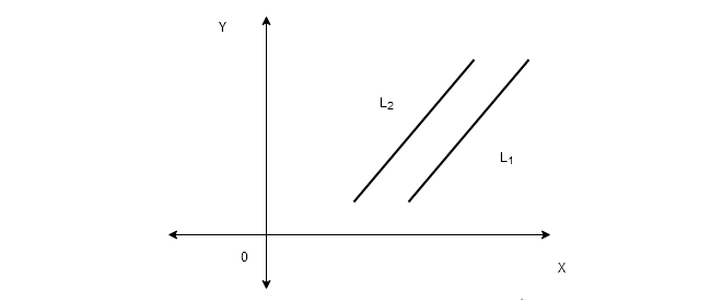
Therefore, the above system has no solution.

Exactly One Solution

Suppose the lines – $L_{1}$ and $L_{2}$ intersect each other exactly at a point $(x, y)$ . Then we have exactly one solution to the linear system.

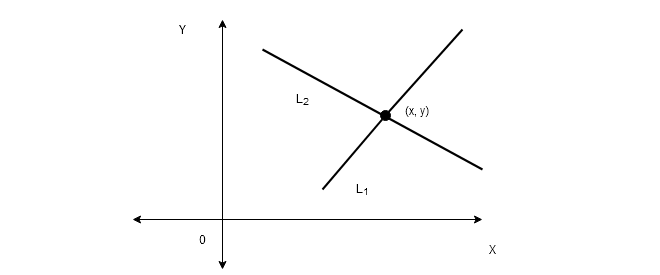
Figure 2 – Linear System With Exactly One Solution

The point $(x, y)$ in the above diagram is the only solution that satisfy equation of both the lines.

Infinite Solutions

When the two lines – $L_{1}$ and $L_{2}$ are the same or overlap each other then we can say that there could be more than one points $(x, y)$ belong to both line.

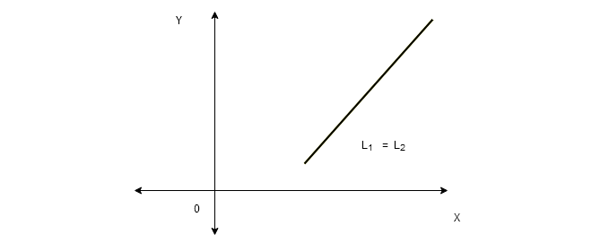
Figure 3- Linear System With Infinite Solutions

Therefore, the equation has infinite solutions because the line may increase forever in the xy-plane. We can formally say that ” Every linear system has no solution, one solution, or infinitely many solutions“.

Augmented Matrix

We know linear equations and system of linear equations from our earlier discussions. Any system of linear equation with $m$ equations and $n$ variable $x_{1}, x_{1}, x_{1}$ , …, $x_{1}$ is written as

\begin{aligned} &a_{11}x_{1} + a_{12}x_{2}+ a_{13}x_{3} = b_{1}\\ &a_{21}x_{1} + a_{22}x_{2}+ a_{23}x_{3} = b_{2}\\ &a_{31}x_{1} + a_{32}x_{2}+ a_{33}x_{3} = b_{3} \end{aligned}

where a’s and b’s are real number constants.

The same equations can be represented using a two-dimensional system called augmented matrix. We usually refer as ‘matrix‘,but the word ‘augmented’ highlights that context of matrix system. We now know from where the matrix came from.

\begin{bmatrix}a_{11} & a_{12} & ... & a_{1n} & b_{1}\\ a_{21} & a_{22} & ... & a_{2n} & b_{2}\\: & : & : & : & :\\a_{m1} & a_{m2} & ... & a_{mn} & b_{m}\end{bmatrix}

The double subscript indicate the correct position of a term with respect to rows and columns where rows are equations and columns are terms.

Important points

Here are some important points to consider while constructing a augmented matrix form a system of equations.

keep the order of a’s according to unknown variables x’s.
keep the b constant on the right in the same order as in the equation.

Example

Problem #1 : Change the following system of linear equations to augmented matrix.

\begin{aligned} &3x_{1} + x_{2}+ 6x_{3} = 1\\ &2x_{1} + 2x_{2}+ x_{3} = 7\\ &4x_{1} - 6x_{2}+ 9x_{3} = 5 \end{aligned}

Solution : The resultant augmented matrix is

\begin{bmatrix}3 & 1 & 6 & 1\\ 2 & 2 & 1 & 7\\ 4 & -6 & 9 & 5\end{bmatrix}

We will consider changing the terms with the help of basic row operations in the next post.

post

System of Linear Equations

Before you we try to understand the system of linear equations, we must understand the basic terminologies that we are going to use in the linear algebra.

Linear Equations

Linear equation represents a straight line on a xy-plane or co-ordinate plane.

a_{1}x + a_{2}y = b

The $a_{1}, a_{2}$ are real number constants and both cannot be zero at the same time.
The $x$ and $y$ are called variables. Hence, the equation is linear equation in variable $x$ and $y$ .

Therefore, linear equation in n variable is given as

a_{1}x_{1} + a_{2}x_{2} + a_{3}x_{3} + \dots + a_{n}x_{n} = b

where $a_{1}, a_{2}, a_{3} \hspace{1ex}$ and $\hspace{1ex} b$ are real number constants.

Examples of linear equations

Here are some examples of linear equations.

\begin{aligned} 3x + 5 = 13\\ \\ \frac{3}{4}y + 3z = 1 \end{aligned}

From the above examples, note that linear equations show following characteristics.

There is not term in the equation with root or product.
All variables are in power of 1.
They do not appear as an argument of another function.

Here are examples of non-linear equations to help you understand the basic differences.

\begin{aligned} &2 + \sqrt{y} = 7\\ &x + 2yz + z = 6\\ &sin \hspace{3px} x + cos \hspace{3px}x = 1 \end{aligned}

Solution Of Linear Equations

A linear equation

a_{1}x_{1} + a_{2}x_{2} + ... + a_{n}x_{n}

has a sequence of $n$ numbers

c_{1},c_{2},..., c_{n}

as solution which satisfy the equation once we substitute them with the variables.

For example,

a_{1}x_{1} + a_{2}x_{2} + a_{2}x_{2} + ... + a_{n}x_{n]} = b\\ \\

The solution is $c_{1}, c_{2},\cdots,c_{n}$
Then,
$a_{1}c_{1} + a_{2}c_{2} + a_{2}c_{2} + \cdots + a_{n}c_{n} = b$ will satisfy the equation.

The set of all solutions of a linear equation is called solution set or general solution to the linear equation.

How to find solution to linear equations ?

Now we will solve two linear equation using substitute method.

Problem #1 : solve $x + 2y = 4$ .

Solution:

We can solve like ordinary algebraic equation. Solve for x for solve for y.

Add $-2y$ to both side of the equation

x + 2y - 2y = 4 - 2y

now we have

x = 4 - 2y

Let’s give an arbitrary value to y. This way we get value for $x$ .

\begin{aligned} &y = 1\\ &x = 4 - 2y\\ &x = 4 - 2\\ &Therefore, \hspace{2mm}x = 2 \end{aligned}

Problem #2 : solve $x_{1} + 3x_{2} - 5x_{3} = 10$
——————————————————————————-

Solution:
————–
This time we can solve for two variables and get the third. We get following equations.

$x_{1} = 10 - 3x_{2} + 5x_{3}$

Let us give arbitrary value to $x_{2}$ and $x_{3}$ .

$x_{1} = 10 - 2(1) + 5(2)$

$x_{1} = 10 - 2 + 10$

$x_{1} = 18$

System of Linear Equations

The system of linear equations is a set of linear equations with $n$ variables $x_{1}, x_{2},x_{3}, \cdots,x_{n}$ .

\begin{aligned} &x_{1} + 5x_{2} + 2x_{3} = 6\\ &3x_{1} + x_{2} - x_{3} = 4\\ &4x_{1} + 2x_{2} + 2x_{3} = 6 \end{aligned}

The solution set $c_{1}, c_{2}, c_{3}, \cdots, c_{n}$ when replaced with variables $x_{1}, x_{2},x_{3}, \cdots, x_{n}$

will satisfy every equation in the linear system. In the above system of linear equations,

$x_{1} = 1, x_{2} = 1$ and $x_{3}= 0$

will satisfy all the equations.

In the next post, we will discuss about inconsistent and consistent system of linear equations.

post