Precedence Graph

A precedence graph is a directed acyclic graph whose nodes corresponds to individual statements.

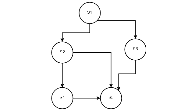
An edge from to , implies that statement can only be executed after statement has completed execution.

In the above diagram following precedence relation is shown:

• S2 and S3 can be executed only after S1 has finished execution.
• S4 can be executed only after S2 has completed execution.
• S5 can be executed only after S2, S3, and S4 have finished execution.

The precedence graph is also a dependency graph.

post

Priority Scheduling

A scheduling algorithms like round-robin treat all processes as same. But if we consider other information about a process, some process is more important than the other. This is the motivation behind priority scheduling.

Each process carries a priority and process with the highest priority will be allocated CPU time. Since there is a chance that the current process may take a long time to finish, the scheduler decreases the priority of currently running with each clock tick. If a higher priority process is found in the ready queue, a process switch happens.

Gantt Chart for Priority Scheduling

Consider the following processes with priority assigned to them.

Process	Burst time	Priority
p1	15	2
p2	3	1
p3	5	4
p4	10	5
p5	4	3

The following Gantt chart shows the new order of process execution.

The waiting time for p2 = 0.
The waiting time for p1 = 0 + 3 = 3.
The waiting time for p5 = 0 + 3 + 15 = 18.
The waiting time for p3 = 0 + 3 + 15 + 4 = 22.
The waiting time for p4 = 0 + 3 + 15 + 4 + 5 = 27.

The average waiting time = (0 + 3 + 18 + 22 + 27)/5 = 70/5 = 14 milliseconds.

Assigning Priority to Process

The priority can be assigned statically or dynamically. For example, UNIX has nice command to change the priority of the user process.

The process priority can be set internally or externally. When it is internal, then all internal factors such a memory, CPU time, number of open files, different ratios, etc are considered. External priority is factors such as the importance of process, department submitting the job, the fund allocated for computing resources, political factors and so on.

The processes can I/O bound, that means it takes most of its time at the device queue. If currently running CPU bound process takes time, then I/O bound process has to wait long time for CPU which is not necessary because these I/O processes have small CPU bursts. Hence, we can safely say that larger the CPU burst, lower the priority and lower CPU burst gets the higher priority.

A simple algorithm to set priority is q/f, where f the fraction of quantum that the process used. If 1 ms is used by the process with 50 ms, then its priority is 50. If 25 ms is used by the same process, its priority is 2.

You may group the process into priority classes and then set the round-robin algorithm on the class for scheduling.

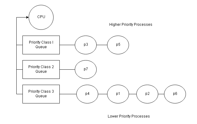
If the CPU only runs higher priority processes, then the lower priority process never gets the CPU time and this results in starvation or indefinite blocking of lower priority processes.

A solution to this problem is aging where we priority is adjusted for lower priority processes waiting for a long time.

References

• Abraham Silberschatz, Peter B. Galvin, Greg Gagne (July 29, 2008) Operating System Concepts, 8 edn., : Wiley.
• Tanenbaum, Andrew S. (March 3, 2001) Modern Operating Systems, 2nd edn., : Prentice Hall.

post

Shortest-Job-First ( SJF )

The shortest job first algorithm associates the length of the next CPU burst with each process. The CPU time is assigned to a process with the smallest next CPU burst time.

Gantt Chart for SJF

If there are two processes with the same next CPU burst time, then FCFS algorithm is applied to them. Consider an example, where the following processes arrived with CPU burst times.

Process	CPU Burst
p1	6
p2	8
p3	7
p4	3

Now we schedule the process according to smallest next CPU burst time. The new process order is in the following figure.

The p4 has waiting time = 0 ms
The p1 has waiting time = 0 + 3 = 3 ms
The p3 has waiting time = 0 + 3 + 7 = 10 ms
The p2 has waiting time = 0 + 3 + 7 + 16 = 26 ms

The average waiting time = (0 + 3 + 10 + 26)/4 = 39/4 = 9.75 ms

Comparison with FCFS

The average waiting time for FCFS would be more than SJF.

Average waiting time using FCFS = (0 + 6 + 14 + 21) = 41/4 = 10.25 ms

The SJF reduces the average waiting time of processes, it is hard to predict the next CPU burst time. But it can be implemented at the long-term scheduler lever where users can submit the process time limit while submitting the job. The CPU scheduler can predict an approximate value of the next CPU burst from the length of previous processes.

References

• Abraham Silberschatz, Peter B. Galvin, Greg Gagne (July 29, 2008) Operating System Concepts, 8 edn., : Wiley.
• Tanenbaum, Andrew S. (March 3, 2001) Modern Operating Systems, 2nd edn., : Prentice Hall.

post

Round Robin

The round-robin scheduling algorithm is suitable for time-sharing computers which are similar to FCFS. However, preemption is added to this algorithm to switch between processes.

A time slice is defined called time quantum which is typically 10 to 100 milliseconds. The processes are allocated CPU time up to 1-time quantum. Then the process is preempted and the next process is allocated the CPU.

A first in first out (FIFO) queue is enough to implement the round-robin algorithm. The FIFO queue must be circular because the processes are added to the tail of the ready queue frequently unless it has terminated before it could complete its time quantum.

Gantt Chart for Round Robin

Consider an example, the following processes arrive at time 0.

Process	CPU Burst
p1	20
p2	5
p3	4
p4	8

Let the time quantum be 4 milliseconds, then

Therefore,

The waiting time for p1 = (25 – 20) + (16 – 4) = 5 + 12 = 17
The waiting time for p2 = 20 – 8 = 12
The waiting time for p3 = 8
The waiting time for p4 = 21 – 16 = 5

The average waiting time = 17 + 12 + 8 + 5 = 42/4 = 10.5 ms

Performance Analysis

The performance depends on the size of the time quantum. If the time quantum is very large the performance is same as FCFS. If the time slice is too small the processor shall take more time to do context switching.

For example, if quantum is 4 ms and context switching task takes 1 ms, then 20% of the time is lost in administrative tasks. Suppose if quantum is 100 ms, then the loss would be 1% of the time.

Now, each process takes 100 milliseconds and if 10 at least are waiting in the ready queue and each one takes 100 milliseconds then the last one takes 1 second which is slow in processor terms.

What if the quantum size is larger than CPU burst? In that case, there would not be a preemption and process will be blocked and the context switch will happen.

The size of quantum should be at least 20 – 50 milliseconds which is neither too high, nor too low.

References

• Abraham Silberschatz, Peter B. Galvin, Greg Gagne (July 29, 2008) Operating System Concepts, 8 edn., : Wiley.
• Tanenbaum, Andrew S. (March 3, 2001) Modern Operating Systems, 2nd edn., : Prentice Hall.

post

First Come, First Served (FCFS)

The first come first served (FCFS) is the simplest CPU-scheduling algorithm. The process which requests CPU first will be allocated CPU first and so on.

The process enters the ready queue and its PCB is linked to the tail of the queue. When the CPU is free, it is assigned a new process from the head of the queue. The FCFS scheduling can be managed with a first in, the first queue. Also, its code is simple to understand.

Example: consider a set of processes arrive at time 0, with burst time in milliseconds.

Process	Burst Time
p1	20
p2	5
p3	10
p4	30

The order in which process arrives is p1, p2, p3, and p4.

The wait time for p1 = 0
The wait time for p2 = 20 + 0 = 20
The wait time for p3 = 5 + 20 + 0 = 25
The wait time for p4 = 10 + 5 + 20 + 0 = 35

Therefore, the average wait time is (0 + 20 + 25 + 35)/ 4 = 80/4 = 20 milliseconds.

Now consider the order, p2, p3, p1, and p4.

The wait time for p2 = 0
The wait time for p3 = 0 + 5 = 5
The wait time for p1 = 0 + 5 + 10 = 15
The wait time for p4 = 0 + 5 + 10 + 20 = 35

Therefore, The average wait time is (0 + 5 + 15 + 35)/4 = 55/4 = 13.75 milliseconds.

The average wait time in FCFS is greater than other algorithms. Suppose there is a single big CPU bound process and many I/O bound processes. If a CPU bound process takes time while all I/O bound process finish their I/O operations and wait in ready queue for CPU. This will lead to an idle I/O device.

The CPU-bound process finishes and goes to I/O queue and all the I/O bound processes whose CPU bursts are small finishes and goes back to I/O devices. The CPU remains idle at this time.

This is a convoy effect where a big process causes other processes to wait and results in lower CPU and device utilization. The FCFS scheduling is non-preemptive, once CPU is allocated, the process remains in CPU until released.

References

• Abraham Silberschatz, Peter B. Galvin, Greg Gagne (July 29, 2008) Operating System Concepts, 8 edn., : Wiley.
• Tanenbaum, Andrew S. (March 3, 2001) Modern Operating Systems, 2nd edn., : Prentice Hall.

post

Types of Schedulers

The multi-programming technique wants high CPU utilization by executing some process all the time. The time-sharing computer keeps switching among processes so that all users can interact with their running programs.

A process scheduler does the selection of processes for execution on CPU. But there are challenges in multi-programming, if a process has to wait for an event, all other processes must wait for it to finish. The bigger the process, longer the wait time and idle time for CPU.

Scheduling Queues

The process that enters the system is put into a job queue. The process already in memory and waiting to execute are put in a list called ready queue. The process executes and quits, or wait for an event such as I/O request. Since many processes do requests for I/O, the processes, therefore, have to wait in the device queue.

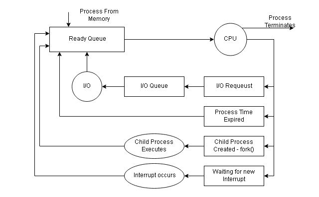
Each device has a device queue.
e.g disk, printer, display, network and so on.

The new process waits in the ready queue until selected for execution or dispatched. Once CPU time is allocated to a process:

• The process can do an I/O request.
• The process creates a new child process and waits for its termination.
• The process can be put back in ready queue forcibly due to an interrupt.

When a process terminates, it is removed from all queues and its resources are deallocated.

Schedulers

A process migrates through various scheduling queues during its lifetime. The selection of processes from queues is performed by the scheduler on behalf of OS.

In batch system, jobs are spooled to a disk for later execution. The job scheduler or long-term scheduler loads processes from this pool to memory.

The short-term scheduler, or CPU scheduler, selects processes from memory that are ready for execution and allocate CPU to one of the processes.

The short-term scheduler switches between processes within milliseconds, therefore, it must be fast enough and not waste time in context switching.

The long term scheduler executes slowly and several minutes before a new process is created. It controls the degree of multi-programming. The degree of multi-programming must be stable – the rate of process creation must equal to rate at which process departs.

When a process departs, the long-term scheduler makes a careful selection of processes to be loaded into memory. The selection is a mix of I/O bound process and CPU bound. If selection is all I/O bound processes, then CPU queue will be empty and it remains idle. If all selection is CPU bound, then I/O queue will be empty leave it idle.

Sometimes operating systems does not have long termscheduler and directly load the processes in memory . Example. UNIX and Microsoft Windows.

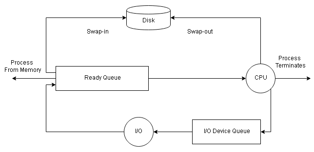
But operating system uses a swapping technique, called the medium-term scheduler. The waiting or blocked processes can be swapped out or swapped into a disk to free memory for other active processes.

References

• Abraham Silberschatz, Peter B. Galvin, Greg Gagne (July 29, 2008) Operating System Concepts, 8 edn., : Wiley.
• Tanenbaum, Andrew S. (March 3, 2001) Modern Operating Systems, 2nd edn., : Prentice Hall.

post

Process Scheduling Criteria

The single processor system, one process runs, and other processes wait until CPU is free. In a multiprocessor system, some process always runs and thus increases the CPU utilization.

If a process is waiting for the completion of some task, or I/O request, the CPU remains idle. To stop wasting CPU time, the CPU switch from the current process to another process. The CPU is one of the computer resources hence it must be scheduled in such a way that we get maximum performance.

CPU-I/O Burst Cycle

The process execution consists of CPU cycle and then followed by an I/O burst cycle, another CPU burst cycle, then followed by I/O burst cycle and so on. Finally, the CPU gets a request to terminate the execution.

IO bound process will have many long I/O bursts and short CPU bursts. A CPU bound process will have a few long CPU bursts and short I/O bursts. This affects the choice of the CPU scheduling algorithm.

CPU Scheduler

When CPU becomes idle the OS must select one of the processes from the ready queue with the help of a short-term scheduler or CPU scheduler.

The ready queue can be implemented using different data structures – a FIFO queue, a linked-list queue, or a tree and so on. The records in the queue are process control blocks (PCBs) of the processes.

Preemptive Scheduling

CPU-Scheduling decision may take place under 4 circumstances:

1. Process switches from running to wait state. e.g IO request.
2. Process switches from running to ready state. e.g interrupts.
3. Process switches from wait to ready state. e.g IO for process completed.
4. Process terminates.

We can ignore 1 and 4 because there is no chance of scheduling. It is called nonpreemptive or cooperating scheduling scheme. When 2 or 3 happens, it is called preemptive scheduling.

Non preemptive scheduling

Process keeps CPU until it is terminated or goes to waiting state.

Preemptive scheduling –

Process can be preempted any time. E.g two process access shared data, one process can be preempted to let others access the data. The preemption affects the design of the OS kernel because a process can be preempted in the middle of the system call, before a context switch. The kernel data structures will be an inconsistent state.

Dispatcher

The dispatcher is part of CPU-scheduling that gives control of CPU to the process selected by short-term scheduler.

This function involves the following:

– Switching context
– Switching to user mode
– Jumping to a proper location in the user program to restart the program.

The time taken to stop one process and start another process running is called dispatch latency.

Scheduling Criteria

We must compare CPU-Scheduling algorithms based on following criteria:

CPU utilization – It is to keep CPU busy that range from 40 to 90 percent.

Throughput – Number of processes completed per unit of time.

Turnaround time – It is the sum of time spent – waiting to get into memory, waiting in ready queue, executing in the CPU, and doing I/O.

Waiting Time – Scheduling gets affected by time spent waiting in ready queue. This whole time spent is called the waiting time.

Response time – Turnaround time depends on output device. But in some interactive systems, you get the first response after process submission although the process may still be working. This time is called response time.

Scheduling tries to maximize :

• Throughput
• CPU utilization

Scheduling tries to minimize:

• Response time
• Waiting time
• Turnaround time

The goal here is to reach an optimize level of performance, rather than maximizing or minimizing any thresholds. You will learn more about this in future articles.

References

• Abraham Silberschatz, Peter B. Galvin, Greg Gagne (July 29, 2008) Operating System Concepts, 8 edn., : Wiley.
• Tanenbaum, Andrew S. (March 3, 2001) Modern Operating Systems, 2nd edn., : Prentice Hall.

post

Message Passing System

In this article, you will learn another popular method of interprocess communication called message passing. You will learn different techniques and characteristics of message passing.

Message Passing

The cooperating processes can communicate with the help of a message passing facility. There are different ways communication happens:

• Between same threads of a process.
• Between processes on same node or computer.
• Between two processes on different nodes or computers.
  Example: chat system over Internet

A message-passing system has atleast two primitive operations:

1. send(message)
2. receive(message)

The messages could be of a fixed size or a variable size. If system uses fixed size messages, then system level implementation is easy. If chosen variable size messages, the system level implementation is difficult, but the programming level task is easy.

If P and Q process wants to communicate, then a communication link must exist between them. There are several ways to implement physical link( shared memory, hardware, or network), but we are interested in logical implementation of a link. Here are different ways to communicate using message passing:

1. Direct or Indirect communication
2. Synchronous or asynchronous communication
3. Automatic or explicit buffering

Direct Communication

Under direct communication, processes must explicitly name the sender or receiver in the communication.

The send() and receive() are defined as:

send(P, message) - send a message to process P
receive(Q, message) - receive a message from process Q

The communication link in direct communication has the following properties:

• The link is established automatically. Processes need each other’s identity to send messages.
• A link is associated with exactly two processes.
• Between two processes, there is only one link.

There is a symmetry in addressing. In asymmetrical addressing, the sending process needs to address the receiver, but the recipient does not need to address the sender.

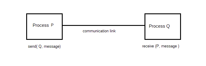
Example of messaging with receiver does not need address of sender.

send(P, message) - send message to P
receive(id, message) - receive message from any process. Id is replaced with name of the sender process.

The disadvantage in symmetric and asymmetric schemes is in changing the identifier of a process. We need to change all the other process definitions and references to the old identifier and replace with the new one.

Indirect Communication

In indirect communication, messages are sent and received from mailboxes or ports. The processes can place messages into a mailbox or remove messages from them. The mailbox has a unique identification.

Two processes can communicate only if they have a shared mailbox.

send(A, message) - send a message to mailbox A
receive(A, message) - recieve a message from mailbox A

In this scheme, a communication link has the following properties:
1. A link is established between a pair of processes only if both have a same shared mailbox.
2. A link may be associated with more than two processes.
3. There may be different links, with each link corresponding to one mailbox, between pair of communicating processes.

Example: P1, P2 and P3 all share mailbox A. P1 sends message to A, while P2 and P3 execute a receive() from A. Which process will receive the message? The answer depends on one of the chosen method given below:

• Allow link to associated with at-most 2 processes.
• Allow at-most 1 process to execute receive() operation.
• Choose randomly at-most one process to receive message or choose an algorithm to receive messages such as round-robin(each process take turn to receive message).

The mailbox may be owned either by a process or by the OS.

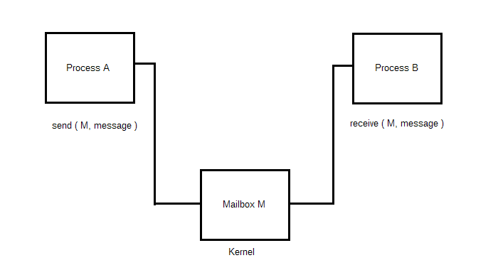
If process owns (mailbox part of process address space) then:

• Distinguish between owner(can only receive through own mailbox), and
• the user (can only send messages to the mailbox).
• When process with mailbox terminates, mailbox disappears, and all other processes should be notified.

If OS owns the mailbox, then:

• It is independent process, not attached to a process.
• Then the OS must allow the process to:

1. create a mailbox.
2. send and receive messages through mailbox.
3. delete the mailbox.

• Process becomes the owner of new mailbox by default.
• Owner process can only receive messages through this mailbox.
• Ownership and receiving privileges can be passed using system calls to other processes.This will result in multiple receivers for each mailbox.

Synchronous and Asynchronous Communication

Communication happens using send() and receive(). There are many options for these two primitives. Message passing may be blocking or non-blocking also known as synchronous and asynchronous.

• Blocking send – sending is blocked, until a message is received by receiving process or mailbox.
• Non-blocking send – sending process sends the message and resumes operation.
• Blocking receive – receiver blocks until a message is available.
• Non-blocking receive – the receiver retrieves either a valid message or a null.

Automatic and Explicit Buffering

The messages exchanged between communicating processes resides in a temporary queue. The queue can be implemented in three way:

1. Zero capacity – with zero capacity the link cannot have messages waiting. Blocking send is the correct option.
2. Bounded capacity – the queue is of finite length n. If queue not full, sender can continue to send messages. If full, blocking send.
3. Unbounded capacity – Infinite queue length; any number of messages wait and sender never blocks.

Zero capacity is called no buffering and other systems called automatic buffering.

References

• Abraham Silberschatz, Peter B. Galvin, Greg Gagne (July 29, 2008) Operating System Concepts, 8 edn., : Wiley.
• Tanenbaum, Andrew S. (March 3, 2001) Modern Operating Systems, 2nd edn., : Prentice Hall.
• I.A.Dhotre (2008) Operating System, Second Edition edn., : Technical Publications.

post

Shared-Memory System

Interprocess communication is necessary to share information between two or more processes. This is how a process cooperates with other processes. In this article, you will learn about one of the two popular models of IPC, which is Shared-memory system.

IPC Models

A process is independent if no affecting or be affected by other processes and does not share data with other processes. A process co-operating if it can be affected or affect other processes. It shares data with other processes.

The cooperating process needs an interprocess communication(IPC) mechanism. There are two models for IPC.

1. Shared Memory – A shared region of memory is established for data exchange.
2. Message passing – communication using message exchanges.

Characteristics of Shared-memory and Message Passing

We have listed a few characteristics for both shared memory and message passing:

• Message passing is used to do smaller messages.
• Shared memory is faster than message passing due to fewer system calls. The message passing system has to call the kernel for each message.
• Shared memory has conflicts when both processes try to access a shared file simultaneously.

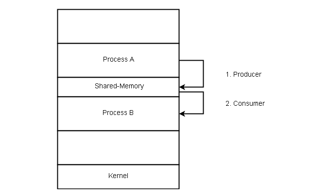
Shared-Memory System

The shared-memory system of IPC needs to establish a shared memory region by the communicating processes. Some characteristics of the shared memory region are:

• Shared memory resides in the address space of the process that creates the shared memory region.
• Another process must add shared address space to their address space to communicate.
• OS does allow address space access by another process, processes must remove this restriction before establishing a shared memory region.
• The processes are responsible for the location, creating, and access to the shared memory reason. OS does not control shared memory region.

Example: The Producer-Consumer Problem

The producer-consumer problem will help understand the concepts of cooperating processes. A producer process produces information consumed by a consumer process.

For example, compiler code makes assembly code consumed by an assembler. A Web server produces HTML, images, etc., and client computers consume the information through the browser.

The producer-consumer problem can be solved by a shared memory region. We must have a buffer of items that is filled by a producer and the buffer emptied by the consumer. The buffer resides in the shared memory region.
The producer and the consumer must be synchronized. While producer creates an item, the consumer consumes another item and not try to consume something not yet created.

The Buffer

The buffer can be of two types:

• Unbounded buffer
• Bounded buffer

Unbounded buffer

• There is no limit on the size of the unbounded buffer.
• The consumer waits for a new item, however, there is no restriction on the producer to produce items.

Bounded buffer

• If the buffer is empty, the consumer must wait for a new item.
• When the buffer is full, the producer waits until it can produce new items.

Let us see how bounded buffer is implemented. A bounded buffer is implemented using a circular queue of an array.

Sample Code #1

#define BUFFER_SIZE 10

typedef struct {
......
} item;

item buffer[BUFFER_SIZE];
int in = 0;
int out = 0;

Consider the producer and consumer code below. The buffer is empty when in == out. The buffer is full when ((in + 1) % BUFFER_SIZE) == out;

Sample Code #2: Producer

item nextProduced;

while (true) {

/* produce an item in nextProduced */
while(((in + 1)% BUFFER_SIZE) == out)
; /* do nothing */
buffer[in] = nextProduced;
in = (in + 1) % BUFFER_SIZE;

Sample Code #3: Consumer

item nextConsumed;

while(true)
{
/* consume an item in nextConsumed */
while(in == out)
; /* do nothing */
buffer[out] = nextConsumed;
out = ( out + 1) % BUFFER_SIZE;
/* consume the item in nextConsumed */
}

The buffer contains BUFFER_SIZE - 1 items and no more.

References

• Abraham Silberschatz, Peter B. Galvin, Greg Gagne (July 29, 2008) Operating System Concepts, 8 edn., : Wiley.
• Tanenbaum, Andrew S. (March 3, 2001) Modern Operating Systems, 2nd edn., : Prentice Hall.

post

Win32 Threads

The Win32 threads are implemented in the kernel space of Windows OS. The multi-threaded applications can use the Win32 API library similar to Pthread library.

We must include Windows.h header file while using win32 API. In the example program below, similar to Pthread – Sum is shared between threads and is the global variable of type DWORD (32-bit integer).

The function Summation () is the second thread created by main thread.

#include <windows.h>
#include <stdio.h>
DWORD Sum; /* data is shared by the threads */
/* the thread runs in this separate function */

DWORD WINAPI Summation(LPVOID Param)
{

DWORD Upper = *(DWORD*)Param;
for(DWORD i = 0;i <= Upper;i++)
SUM += i;
return 0;
}

int main (int argc, char *argv[])
{
DWORD ThreadId;
HANDLE ThreadHandle;
int Param;
/* perform some basic error checking */

if (argc != 2 ) {
fprintf(stderr,"An integer parameter is required\n");
return -1;
}
Param = atoi(argv[1]);
if (Param < 0) {
fprintf(stderr,"An integer >= 0 is required\n");
return -1;
}
//create the thread 
ThreadHandle = CreateThead(
NULL, //default security attributes
0, // default stack size
Summation, //thread function
&Param, //parameter to thread function
0, //default creation flag
&ThreadId); //returns the thread identifier

if (ThreadHandle != NULL){

// wait for thread to finish
WaitForSingleObject(ThreadHandle, INFINITE);

//close the thread handle
CloseHandle(ThreadHandle);

printf("sum = %d\n", Sum);
}
}

The CreateThread() function create the thread when attributes are passed as parameters. The attributes are stack size, a flag to ensure blocking state during thread start, function Summation and its parameters.
The WaitForSingleObject() make parent thread to go to blocking state and wait until Summation () thread is completed.

References

• Abraham Silberschatz, Peter B. Galvin, Greg Gagne (July 29, 2008) Operating System Concepts, 8 edn., : Wiley.
• Tanenbaum, Andrew S. (March 3, 2001) Modern Operating Systems, 2nd edn., : Prentice Hall.

post