Introduction to DBMS
Think about small data like phone numbers of friends, grocery items list, etc. It is easy to store these information on a piece of paper and retrieve when you need them. An individual can manage it well. Now imagine a large organization that store huge number of data year after year. They need to setup an information system that store , update it regularly, secure, reliable and people should be able to retrieve it quickly in an efficient manner. The core of such an information system is the database management system. In short, DBMS.
This database system has a single goal and it is to provide a consistent environment to store, update and efficient retrieval of data in an organized manner. Other operations of database system is to secure the data servers, and take various security measures, give concurrency control to database, which means manage access to database by multiple users at the same time, database recovery in case of crash, or failure of database servers. Its not necessary that data is always stored on a servers, because an information system can contain various types of storage hardware.
Now that you understand core function of a database management system or DBMS. Let’s talk about most important component of this system – the database.
“A database is structured collection of related data”.
I have to elaborate the definition. Here structured collection means that the data is organized in such a manner that it make storage easy, and retrieval efficient and faster.
The word related data is referring to the type of data stored which may be images, records , or database of audio/video files. The data is related because of its shared attributes or common properties that help in categorizing data in the form of a database.
Tasks Performed by a Database
You know what get stored in a database from its definition. To maintain a consistent database with updated information, it has to perform certain tasks. These are
- Add files to database that store information permanently.
- Add data to files in the form of records, relations, and various logical structures.
- Help retrieve data for users and applications including database administrators.
- Update new data.
- Delete data from files.
- Remove database files if necessary.
The tasks are called basic database operations of DBMS. Data record creation, reading data, updating data and deleting data are core functions to maintain databases.
There are other features about database management systems which I will discuss in next sections.
Features of DBMS
In modern database systems , you will find three common features listed below.
- Data Independence
- External Schema or Views
- Query Mechanism
Each of these features enable database operations , manage consistent database , efficient data retrieval and security to database systems. I will briefly discuss each of these features just enough for you to understand and later on I will elaborate on these topics in a different article.
Data Independence
The idea of data independence is very simple idea that we should able to modify database schemas or database levels without affecting the higher level schemas. A schema is structure and organization of the database at three levels.
- Physical Schemas
- Conceptual Schemas
- External Schemas
The physical schemas are related to how database stores information physically, and database indexes for quick searches. The level above physical schema is the conceptual schemas or logical schema. The external schemas are above logical schemas and it is the highest level of three level schema structure.
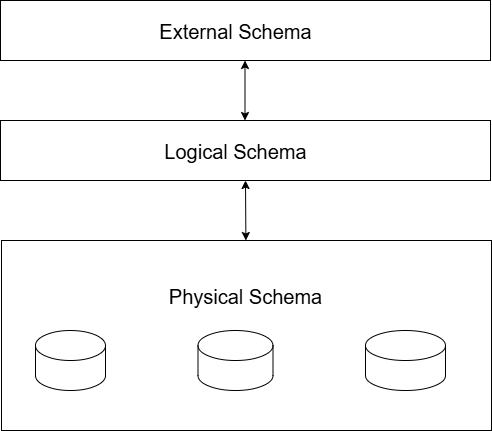
The ability to change the structure of physical schema without affecting higher schemas like logical schema or external schema is called physical data independence. Physical data independence is also called the internal data independence.
DBMS query is a user request to manipulate databases and these user requests are translated / executed using a Structured Query Language (SQL). Each database query must go through three process
Similarly, you can modify or change structure of conceptual schema (logical schema) without affecting the higher external schema which is knowns as logical data independence. If the logical data independence is achieved , it is also external data independence because it does not require you to change the external schemas or user views.
External Schemas or Data Views
The external schema or views are highest level of database abstraction. It simply means that you can create more views or tables from the same database different from logical schema and/or physical schema.
Users of external schema don’t have or want to do anything with how data is stored in the database. A particular external view only shows them, what they need to know. Not only that , but DBMS also allows you to create multiple views from same database.
For example, A bank account holder will see only his account details such as bank balance and transaction history etc. On the other hand, a bank manager will see overall status of accounts and customer personal information. One aspect of view is access privileges’ which decide how much and which views a user get to access. You doing Google search and search results on the page is also a external view , totally different from how Google store websites information.

External schemas can stay the same, yet when application using them or user change the data , that is reflected in the logical schema. This is external data independence.
Another advantage of external schema and its independence from conceptual schema and physical schema is data security. With limited access to information, database administrators can protect sensitive information from threats or unauthorized access.
Query Mechanism (SQL)
- Parsing or Translation
- Execution
- Query Optimization
The Query parsing is a process to check syntax error in SQL command called the syntax checking, then the parser checks for semantic errors meaning does the database and table exists, compatibility of query, etc. If the query is passed all checks, it translate the query to relational algebra or a query tree, both of which are internal representation of query for optimization.
The query optimization is to prepare the query for efficient execution by reducing time and resources to execute the queries. Finally, the query is executed and precise results are fetched.
To understand the advantages of DMBS system let us compare it with older version of database system. There were no systems to store data and earlier database applications were build using the computer file system. In other words, data were stored in files and accessed directly.
File System vs. DBMS
Like file system, DBMS also stores data in files, but it provides a system to manage it well using three tier-schemas. Then there is additional security and concurrency control.
The traditional file system has few problems with storing data which are:
- Duplicates data – sometime files or duplicated entries cause problems with application or users. Sometime users create multiple files with same name or enter duplicate entries that can cause confusion or give erroneous results. In DBMS, each record is given a unique id to prevent duplicates.
- Change in one file is not reflected in other files – Since multiple users access the files and change it continuously, sometimes they are not synced together and you may find difference in data because it is not updated on other files. With DBMS system, change in relations or views, it either Updated or terminated completely.
- Multiple file formats – With traditional file system, files are often stored in multiple formats and that will limit the data independence and increase costs of maintaining such a system.
- Database Integrity problems: Database integrity refers to consistency, accuracy and reliability of database and it is enforced using database constraints which are nothing but rules for databases. With file system, adding constraints or modifying them such as file size, user permissions, etc. With DBMS system, there are fewer constraints management and they are easy to implement.
- Atomicity : DBMS transactions to database are atomic, means they either succeed or fail , so the database is always consistent and safe. With file system, failure of database can leave the database in inconsistent state.
- Concurrent Access Problems: The traditional file system is not good at handling multiple users concurrently accessing the database, two user can access the same data and leave the wrong entry.
- Security: It is very difficult to ensure file security and security constraints in traditional file system.
DBMS Solution to all the above mentioned problems:
- Logical storage reduce space, time to access data and complexity. The logical storage also prevents duplicated and updating time.
- It has indexes to do faster searches and special data structures for faster retrieval of data.
- Simple as well as complex queries through SQL is possible.
- Database Integrity constraints are handled efficiently.
- Backup and Recovery system.
- Database security by restricting users based on roles and permissions. Only authorized users can do certain high level tasks.
- Multiple User Interfaces for different types of users. For example, menu-based, form based interfaces and GUI( graphical user interfaces). There are separate interface for database administrators.
Summary
The DBMS system stores data in organized manner and performs database operations on them such as Add, Update, Delete or Modify.
Database has three-level architectures that provides full data independence. One level need know activities of higher level schemas. Apart from that DBMS is provides database security, concurrency access and backup and recovery system.
Database queries are handled through an easy and simple query language called SQL ( Structured Query Language).
Finally, I mentioned the difference between traditional file system database and DBMS. The solution provided by DBMS is robust and efficient.
Database Management (DBMS) Notes – Concepts, Examples, MCQs & Exam-Ready Revision
Database Management System (DBMS) is a core subject in Computer Science and IT courses as well as competitive exams like GATE, UGC NET and university exams.
On this page, you will find structured resources to learn DBMS concepts, along with clear explanations, examples and exam-ready revision notes.
What will you learn
On this page you will find:
- Core DBMS concepts explained clearly and systematically
- Exam-oriented explanations supported with relevant examples
- MCQ-based practice posts to test your understanding
- Detailed articles along with exam-ready revision PDFs
This Page is for:
- Computer science and IT students
- GATE and other competitive exam aspirants
- University exam preparation
- Self learners
Topic Sections
Find DBMS topics here.
(1) DBMS Fundamentals
(2) ER Model & Database Design
(3) Relational Model
(4) Relational Algebra & Relational Calculus
(5) SQL
(6) Functional Dependencies
(7) Normalization
(8) Transactions
(9) Concurrency Control
(10) Recovery System
(11) Indexing
(12) File Organization
(13) Query Processing
🎁 Get the SQL Starter Kit (Free for Students)
Build your SQL foundation with these three essential PDFs:
- SQL Basics Explained
- MySQL Installation Guide
- SQL Practice Questions (20 problems)
This starter kit is free, but requires a quick signup so we can send the PDFs directly to your inbox.
👉 Sign up and receive the download link instantly
The Three Schema Architechture of Relational database
In relational database system, the three-level architecture describes how users view the data. It separates physical storage details from users and applications. It provides data abstraction and data independence.
Why we need this architecture?
The main reasons for three-level architecture is:
Data abstraction
- Users can access data without knowing the physical storage details.
Data Independence
It means changes in one level does not affect the other levels.
- Logical data independence – It means changes in logical schema (tables, relations) does affect the users or applications.
- Physical data independence – changes in the physical storage (disk, indexes) does not affect the logical tables or relations.
Multiple Views of Same Database
- Different users can view database according to their need and privileges’.
For example, an admin can see tables and he can create a new one if needed, but a common user can only see limited view of data provided by the application, they are using.
Security and Consistent Data
The three-level architectures provides security and data consistency.
- The physical data access is restricted.
- Since, DBMS manages everything from one location, the data is consistent, and there are no duplicate records across multiple copies of the database.
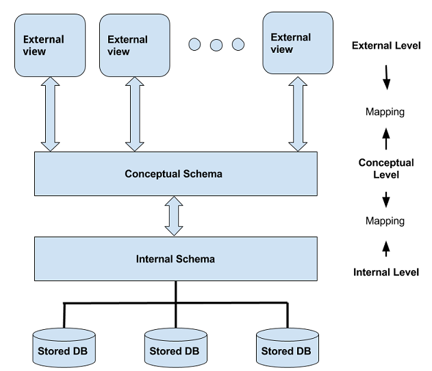
Internal level with internal schema
The internal level is the lowest level of data abstraction. It deals with the physical implementation of the database in a computer system. In other words, it is the physical level.
Storage Structure
It describes how data is organized and stored on a disk storage. There are two main concerns;
- Efficient use of disk space.
- Minimum disk I/O
It is because the disk is slower than the random access memory (RAM) of a computer.
DBMS decides:
- how records are placed in files.
- structure of records, variable length or fixed length.
- how data blocks are arranged.
Only files are part of a file system, where records and blocks are low level details are part of disks. The operating system manage files, file system, blocks and records.
Fast Search and Retrieval of Data
A fast search and retrieval of data is primary concern of physical storage. It is achieved through Indexing. The indexes are added as additional structures at physical level.
The most popular indexing types are:
- B+ trees
- Hash indexes
- Clustered and non-Clustered indexes
The solution is reading data without scanning the whole disk and reducing the disk I/O.
Buffer Management
Buffer is a temporary storage memory, usually, in RAM to hold data, while transferring between to locations or devices. In DBMS, buffer management is an important task.
The buffer pool can hold page table and memory pages.
DBMS do not interact with disk every time. It uses a buffer pool to access data from memory, than accessing disk which is slower process.
The primary concern is to decide which page should remain in memory and which dirty page should sent back to the disk.
Pages are managed with page replacement algorithms such as LRU( Least Recently Used). This directly affect the performance of the database.
Data Security
Data security exists at various levels. At the physical level, the data security is concerned with physical security of infrastructure, servers, etc. This is secured by giving access to only authorized people. Not everyone get the same access permissions. The DBA gets full access to the database.
The main concern for physical security are;
- Data Files
- Disks
- The Backup Disks and Files.
Data files are secured using various encryption techniques. The access control can limit the access to only authorized people to read, write, or modify the data files. Sometimes the files are immediately destroyed if they are no longer required.
Data disk security includes methods like Self-Securing Disks (SSDs), password protection, full disk encryption like FileVault, BItLocker, etc.
Backups are useful incase of loss of data or disks. There two ways to keep backup.
- Local backup
- Offsite back
In either case, backup disks and files need own protection using encryption, access control, and isolating the backup locations.
Even all of these cannot prevent database crash or failures. Next section discuss the integity and recovery of data.
Data Integrity and Recovery
When the database is crashed, our concern is to prevent corruption of physical data and recover the database and any lost data.
This is achieved through transaction logs:
- Write-Ahead-Log (WAL) – Database transactions do not write anything to database because a failure can corrupt database during writing process. Therefore, database transactions follow integrity , atomicity, and durability principles( ACID Properties) and write in the WAL files before they commit the information permanently to the database.
- Checkpoints – A checkpoint in the log files, is a marker that all memory pages are written to the disk and database is consistent. It is used to recover the database to a consistent state.
- Redo/Undo Logs – Redo log store all committed transactions and new values of the data. The Undo logs contains previous versions of data. Database can rollback to previous version if the current transaction fails.
Conceptual Level with Conceptual Schema
In the three-level architecture, conceptual level sits between the external level and the internal level. It describes the logical structure of the complete database regardless of its physical implementation.
Conceptual level is the overall view of the database and it represents all the information going to be represented in the database.
The conceptual level represents;
- What data is stored.
- What is the relationship between data
- Constraints on the data
For example;
Entities – Student , Course, Department
Attributes – StudentID, Name, Grade
Relationship – Students enroll for Courses
This level is usually represented using schemas or models such as Entity-Relationship Models or Relational Model.
What are the main concerns at conceptual level
The main concerns at conceptual level are listed below:
- Logical structure
- Relationship between data
- Data integrity constraints
- Data independence
- Security and Authorization
Logical Structure
The DBMS at conceptual level must clearly define:
- Tables (relations)
- Attributes (columns)
- Keys ( primary key, foreign keys)
The tables with columns are completely different from how physical records are stored. The keys such as primary key and foreign keys ensures that records are not duplicate. The table allows duplicate data if key is not defined.
Example.
Student Table (Student_id, Name, Department_id)
Relationship between data
The table row represents an instance of an entity. Table is entity type , set of all similar entities.
The relationship between data is how entities are connected. These relationships ensure that the database captures real world structures.
For example.
Student enrolls in a Course
Department offers a Course
Data Integrity Constraints
The data in the database must follow rules and precise structure. The correct data is valid, consistent across database, and meaningful according to the constraints.
A consistent data is that which follows all rules, even though duplicate records exist in the database tables.
Common constraints includes:
- Primary key to uniquely identify records.
- Foreign key to maintain relationships.
- Domain constraints to ensure valid values for attributes.
For example:
In Student Table, Student_id cannot be NULL due to constraint NOT NULL on that field. Student_id can be a Primary Key that uniquely identify the Student Table, therefore, NOT NULL make sure that all students have an ID.
Data Independence
The most important job of conceptual level is to hide the physical storage details from the users. If the storage structure change, a disk, or index, it does not affect the conceptual level. The conceptual schema does not change.
This is called logical data independence.
Security and Authorization
At conceptual level, we are dealing with different types of data. The data is modified, read and deleted. In short, there are many database operations on this data.
Conceptual level decides
- Who can access which data?
- User permissions.
For example,
Students can view their Grades, however, only administrator can modify the Grades.
What is the role of a Conceptual Schema ?
The conceptual schema is the blueprint of the database. It acts like a bridge between external level(user views), conceptual level (logical structure), and internal level (physical storage) of the database.
The overall organization of the data is independent of the physical storage.
External or View level
The external level is the top-layer of the three-schema DBMS architecture. It does not show full database, only relevant part of data to a single user or an application. This is called Views.
For example,
There can be a Student view with fields – Student Name and Grade.
There can be one view for Admin with following fields – Student_id, Name, Grade, Fees.
It is same database , and tables structure but different views for different people.
What are the main concerns of External level?
External level interacts with users. It has different concerns than conceptual and internal level.
- Data abstraction
- Security and Access Control
- User-Specific Views
- Data Independence
Data Abstraction
The main goal of external views is to provide necessary data to the users. Users don’t need to see the internal database structures or physical implementation of DBMS.
Hiding the important database details is the first priority of external views.
For example.
A student only need to see the marks obtained, they don’t need to see the table design, or change anything in the database. A view is generated with only student ID, Name and Marks.
This indicates the security and authorization problems which is discussed in the next section.
Security and Access Control
Security and authorization is most important here. Unauthorized users should not get access to information. The admin protects the views with secured passwords. Every user get their own password and only they are authorized to view the data.
All sensitive data is hidden. Users get only authorized information.
User-Specific Views
User-specific view is customized representation of database that contains only the data a particular user (or role) need.
The views are filtered vertically, then only relevant columns of tables are shown.
Similarly, view are also filtered horizontally, where user can see only specific records.
For example.
Students can see only own records.
Manager can see only his department records.
Data Independence
Change in the internal or conceptual level does not affect the external view. The users will never notice any change happening in database. This is called external data independence.
Summary
| Level | Key focus | Describes | Users |
| External | User view | Different views of data for different users. | Common end users |
| Conceptual | Logical Structure | Logical design of database (Table, Relations) | DB Designers, DBA |
| Internal | Physical Storage | Storing data on disk (File, Indexes) | System/DBMS |
How to Add a Constraint and Remove a Constraint From a Relation?
Constraints are like rules in relation so that you cannot violate them. There are plenty of constraint types that we use. In this article, we will add a check constraint and delete it from a relation.
The general process to add or remove a constraint from a Relation is as follows.
STEP 1:
In this step, you create EMPLOYEE relation and put a check constraint on Gender.
CREATE TABLE EMPLOYEE (EMPNO NUMBER(5) PRIMARY KEY, ENAME VARCHAR2(20), GENDER CHAR(2), SALARY NUMBER(7,2));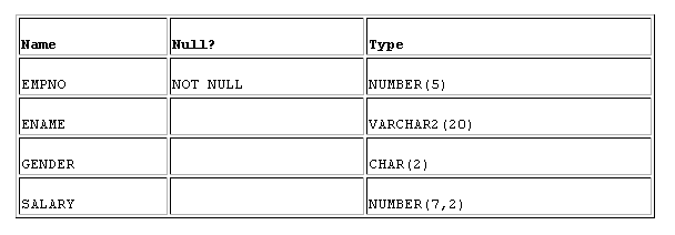
STEP 2:
Here we add the constraint to the table .
ALTER TABLE EMPLOYEE ADD CONSTRAINT CHK CHECK (GENDER IN( 'M','F'));
STEP 3:
Now, you are going to delete the constraint, but before you drop the constraint, let us show you, how to get the constraint name first.
It is a necessary step if you are not the DBA who created the constraint on the relationship and you cannot delete the constraint unless you have appropriate permission.
SELECT CONSTRAINT_NAME FROM USER_CONSTRAINTS WHERE TABLE_NAME = 'you table name';In the above command, you only need to change the “Your Table Name’ with a table name that exists. In this example, EMPLOYEES.
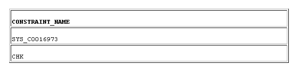
STEP4:
Now that I have the name of the constraint , We can delete the constraint using following command.
ALTER TABLE EMPLOYEE DROP CONSTRAINT CHK;
Summary
Following the above four steps can help you to identify and remove the constraints set on your database tables. Note that these commands are performed on Oracle 10g, therefore, you must be careful while running the same on other database systems. The command and procedure may be different.
Understanding GROUP BY and HAVING Clause
We use SELECT-FROM-WHERE kind of statement to run queries that get us specific rows from a relation. In the select statement, WHERE is the condition that returns specific rows from a relation.
What if we want to group the information? The GROUP BY and HAVING clause helps you to group the resultant rows by a specific column. GROUP BY and HAVING clause is used with aggregate functions like Count, Max, Min, Sum, etc;
This is easy to understand with an example.
Step 1:
Create a relation for students – Student ( rollno, name, age);
CREATE TABLE STUDENT (ROLLNO NUMBER(5) PRIMARY KEY,NAME VARCHAR2(30), AGE NUMBER(3), GRADE CHAR(2));
STEP 2:
Enter details of at least 10 students in to the STUDENT relation.
INSERT INTO STUDENT VALUES(50001,'DHANUSH',39,'A');
INSERT INTO STUDENT VALUES(50002,'RAJNI',29,'D');
INSERT INTO STUDENT VALUES(50003,'VIKRAM',32,'S');
INSERT INTO STUDENT VALUES(50004,'VADIVEL',25,'D');
INSERT INTO STUDENT VALUES(50005,'PRASAD',37,'S');
INSERT INTO STUDENT VALUES(50006,'SHANKAR',21,'A');
INSERT INTO STUDENT VALUES(50007,'RAM',33,'A');
INSERT INTO STUDENT VALUES(50008,'KARTICK',22,'C');
INSERT INTO STUDENT VALUES(50009,'SHAKTI',35,'B');
INSERT INTO STUDENT VALUES(50010,'SIMBU',20,'B');
To check the entered value in the table, you can run following query against the STUDENT relation.
SELECT * FROM STUDENT.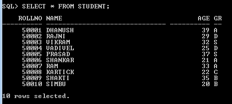
STEP 3:
You can run two simple queries to understand the difference between a query without group by and a query with GROUP BY clause. First, you want a student with minimum age from the STUDENT relation using an aggregate function MIN().
SELECT MIN(S.age) FROM STUDENT S;You can add WHERE clause, but we want query without any conditions. It will produce the following results.
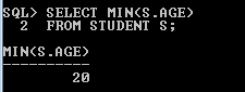
You can see that there is only one person in an entire student relation whose minimum age is returned.Suppose you want to write a query to get the minimum age of student by student Grade. It means this statement “What is the minimum age of students who got A’s ?” or “What is the minimum age of students who got B’s?” and so on.
Let’s run the following query that will get you the minimum age grouped by student GRADE.
SELECT S.GRADE, MIN(S.age) FROM STUDENT S GROUP BY S.GRADE;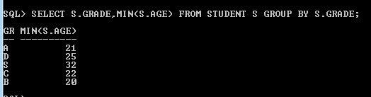
What is the Difference ?
In the first query, we treated the entire STUDENT relation as one group and that’s why we only have a single value for the whole relation.In the second query, we grouped STUDENT relation by student grade and for each of these grade got minimum age.
The HAVING clause
The HAVING clause is qualification for the Group By clause. It means you are putting more conditions on the resulting rows from GROUP BY clause.
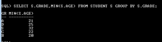
SELECT S.GRADE, MIN(S.age) FROM STUDENT S GROUP BY S.GRADE;You know that it will return a list of minimum age by student grade, but suppose you want to see only minimum age that are greater than or equal to 30.
SELECT S.GRADE, MIN(S.age) FROM STUDENT S GROUP BY S.GRADE HAVING MIN(S.age) >= 30;The result is only one row whose minimum age is greater than or equal to 30 but grouped by student grade.
Group by cannot have duplicate values and the general format of the query is given below.
SELECT [DISTINCT] select list
FROM from-list
WHERE qualification
GROUP BY group-list
HAVING group-qualification
Source: Database Management Systems – Raghu Ramakrishan
You want to understand the GROUP BY and HAVING clause, then create similar examples and run them against the relations.
🎁 Get the SQL Starter Kit (Free for Students)
Build your SQL foundation with these three essential PDFs:
- SQL Basics Explained
- MySQL Installation Guide
- SQL Practice Questions (20 problems)
This starter kit is free, but requires a quick signup so we can send the PDFs directly to your inbox.
👉 Sign up and receive the download link instantly
JOIN Concepts in Relational Database Management System
JOIN put condition (selections and projections) on a CROSS-PRODUCT from two or more tables and the result is a smaller relation than the CROSS-PRODUCT
In DBMS, JOIN is an important operation in relational algebra and it extracts useful information from joining two or more relations. In this lab, you will create two tables TEACHER and STUDENT. A STUDENT studies under one or more TEACHER for different subjects, so student and teacher have a One-to-Many relationship.
Step 1: Create Table TEACHER and STUDENT.
Before we dive into the JOIN concept let’s create relations – TEACHER and STUDENT. You have to use the following SQL commands to do that. In the relations, TEACHER, and STUDENT, the TID and SID are primary keys respectively.
CREATE TABLE T (TID NUMBER(5) PRIMARY KEY , CNAME VARCHAR2(30));
CREATE TABLE STUDENT ( SID NUMBER(3) PRIMARY KEY, SNAME VARCHAR2(30), TNAME VARCHAR2(25), GRADE CHAR);
Step 2: Insert values into both the tables as follows
The next step is to insert values into both relations. First, you need to enter values for the TEACHER relation using following command,
INSERT INTO TEACHER VALUES(10001,'RAMESH');
INSERT INTO TEACHER VALUES(10002,'KIRAN');
INSERT INTO TEACHER VALUES(10003,'JOHN');
INSERT INTO TEACHER VALUES(10004,'PETER');
INSERT INTO TEACHER VALUES(10005,'FRODO');
An instance of TEACHER relation is given below.
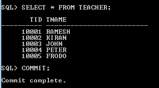
Insert values into the STUDENT table as follows.
INSERT INTO STUDENT VALUES(501,'ANIL KUMAR' ,'RAMESH','S');
INSERT INTO STUDENT VALUES(502,'RAJESH KAPOOR','KIRAN','D');
INSERT INTO STUDENT VALUES(503,'SUBBARAJ','JOHN','A');
INSERT INTO STUDENT VALUES(504,'NAGESH ','PETER','C');
INSERT INTO STUDENT VALUES(505,'RAM PRASAD','FRODO','A');
INSERT INTO STUDENT VALUES(506, 'JASSE');
INSERT INTO STUDENT VALUES(507,'MADHU');
An instance of relation STUDENT is shown below, you must get similar results. For each student there is a teacher associated who taught a course.
The course relation is not required at this moment because these two relations are sufficient to understand the JOIN concepts in DBMS.
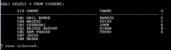
Cross-Product (Cartesian Product)
A Cross-Product is a product of two or more relations and is denoted by T ⨯ S. Suppose the relation Teacher has 5 tuples and the relation Student has 4 tuples, then the Cross-Product will have 5 x 4 = 20 tuples. Cross-Product is a JOIN without any conditions.
The Cross-Product operation results in a very large relation with multiple tuples. The JOIN operation accepts some conditions and applies them to the Cross-Product and result is a relational instance you want.
Depending on the condition applied you get different types of JOIN.
Note: A Cross-Product is also called NATURAL JOIN.
Equi-Join
SELECT * FROM TEACHER T, STUDENT D WHERE T.TNAME = D.TNAME;This will return all the rows that are common in both teacher and student table.
i.e. t.tname = d.tname.

Left-Outer Join
In this join type, you get all rows that are common to both tables, (EQUI-JOIN) + remaining row from the left side table.
for example
SELECT T.TID,T.TNAME,S.SNAME, S.GRADE FROM TEACHER LEFT OUTER JOIN STUDENT ON T.TNAME = S.TNAME;In the above command the TEACHER is left table and student is right table.

Right-Outer Join
In this type of JOIN, you get all row that are common to both table (EQUI-JOIN) + REMAINING ROWS from right side table.
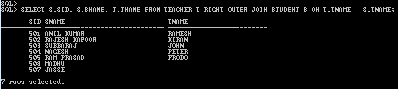
SELECT S.SID, S.SNAME, T.TNAME FROM TEACHER T RIGHT OUTER JOIN STUDENT S ON T.TNAME = S.TNAME;The student table is right hand side table, and you get most of your column from right hand side table. It means that the query returns rows that are in both table + rows in student table only.
🎁 Get the SQL Starter Kit (Free for Students)
Build your SQL foundation with these three essential PDFs:
- SQL Basics Explained
- MySQL Installation Guide
- SQL Practice Questions (20 problems)
This starter kit is free, but requires a quick signup so we can send the PDFs directly to your inbox.
👉 Sign up and receive the download link instantly
Converting an E-R Model into Relational Model in DBMS
In this lesson you will learn to convert er model into relational model. First step in designing a database is to create an entity-relationship model. Then the entity-relationship model is converted into a relational model.
The relational model is nothing but a group of tables or relations that create for your database.
Read: DBMS Basics
Read: Basic DML commands
Read: Basic DDL commands
This article you will learn to convert an entity-relationship model into a relational model using an example. You will understand the process of modeling the real-world problem into an entity-relationship diagram and then convert that entity-relationship diagram into a relational model.
Problem Definition
In this example problem, you will create a database for an organization with many departments. Each department has employees and employees have dependents. To create a database for the company, read the description and identify all the entities from the description of the company.
- The company organized into departments and departments have employees working in it.
- Attributes of Department are dno, dname. Attributes of Employee include eno, name, dob,gender, doj, designation, basic_pay, panno, skills. Skills are multi-valued attribute.
- The Department has a manager managing it. There are also supervisors in Department who supervises a set of employees.
- Each Department enrolls a number of projects. Attributes of Project are pcode, pname. A project is enrolled by a department. An employee can work on any number of projects on a given day. The Date of employee work in-time and out-time has to keep track.
- The Company also maintains details of the dependents of each employee. Attributes of dependent include dname, dob, gender and relationship with the employee.
Model an entity-relationship diagram for the above scenario.
Solution – Converting ER model into Relational model
From the real-world description of the organization, we were able to identify the following entities. These entities will become the basis for an entity-relationship diagram or model.
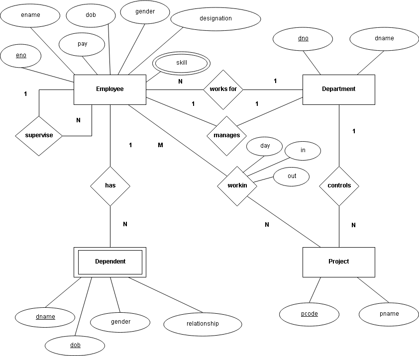
Convert to Relational Model
The next step in the database design is to convert the ER Model into the Relational Model. In the Relational Model, we will define the schema for relations and their relationships. The attributes from the entity-relationship diagram will become fields for a relationship and one of them is a primary field or primary key. It is usually underlined in the entity-relationship diagram.
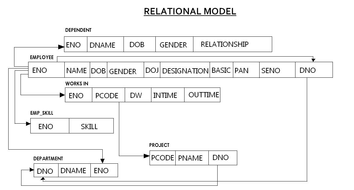
An entity in a relational model is a relation. For example, the entity Dependent is a relation in the relational model with all the attributes as fields – eno, dname, dob, gender, and relationship.
Here is the Relational Model for above diagram of the company database. This the result after converting ER model into relational model.
References
Avi Silberschatz, Henry F. Korth, and S. Sudarshan. 27-Jan-2010. Database System Concepts. McGraw-Hill Education.
Ramakrishnan, Johannes Gehrke, and Raghu. 1996. Database Management Systems. McGraw Hill Education; Third edition (1 July 2014).
Understanding Basic SQL Queries in DBMS
Data Manipulation Language ( DML ) is the language used to maintain the database in a DMBS. The SQL (Structured Query Language) is the most popular language to manipulate databases.
DML Commands
The DML commands perform following tasks on a database.
- INSERT
- SELECT
- DELETE
- UPDATE
The SQL being a DML can do above task without any problem. Other than inserting, deleting or querying database, the SQL has advanced commands to change the schema of relations or create new relations.
It is used for maintaining the database and they are called Data Definition Language (DDL) commands. You can create table, delete a table and do other operations to maintain the structure of your database.
INSERT command
The INSERT command helps insert data into the relation. For example, you can insert values in the ‘MANAGER’ relation as follows.

The schema for Manager relation is given in the previous post about DDL commands.
SELECT command
The SELECT command helps query the database and retrieve the tuples from one or more relations.
There are two types of query – Selection(σ) and Projection(π).
Selection(σ)
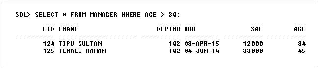
This unary operator selects all the tuple in a relation that meet specific condition using normal conditional operators and logical operator such as AND, OR and NOT.
For example
 , will return all the tuples that have an age greater than 30.
Projection(π)
This unary operator selects columns, but you can add selection with those retrieved columns.
For example
 will return two column – age and salary.

Rename operator(ρ)

The rename operator will rename the existing field of a relation to a different specified name. Alter is a DDL command that modifies the relation name.

UPDATE command
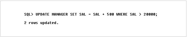
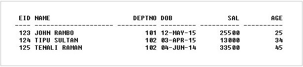
The UPDATE command modifies the value for one or more tuple in the relation. In the following example, we have an updated salary of a manager whose salary is less than 20000.
The result of the update is as follows.
DELETE command

The DELETE will delete the tuple from the relation. Here is an example of DELETE.
The following figure shows the relation Manager after the delete operation. Note that one entry is already deleted successfully.

🎁 Get the SQL Starter Kit (Free for Students)
Build your SQL foundation with these three essential PDFs:
- SQL Basics Explained
- MySQL Installation Guide
- SQL Practice Questions (20 problems)
This starter kit is free, but requires a quick signup so we can send the PDFs directly to your inbox.
👉 Sign up and receive the download link instantly
Basic Data Definition Language(DDL) Commands
The Data Definition Language( DDL ) commands are used for creating new or modify existing schema of a relation. You can also set constraints such as key constraints, foreign key constraints, etc on a relation.
CREATE TABLE Command
This command creates a new relation or table. You must specify the fields and data type for each field while using this command.

ALTER TABLE Command
This is most important of DDL commands because it allows us to modify the table anytime.
Here are some examples of ALTER TABLE command
Adding a primary key for the table. A primary key uniquely identifies a tuple in a relation.

Adding a foreign key for the table. A foreign key in a relation refer to primary key of another relation and cannot be null called the Referential Integrity.

In the above example, we receive an error because the attribute ‘DEPTNO’ is not set as primary key in relation to ‘EX_DEPT’.
After adding ‘DEPTNO’ as primary key we are able to set the foreign key for ‘MANAGER’ relation.

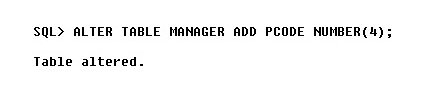
Adding a new column in a Table. In the following example, we are adding ‘PCODE‘ in the ‘MANAGER’ table.
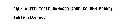
Removing a column from a relation or table. In the following example, we are removing the ‘PCODE’ column from the ‘MANAGER’ table.
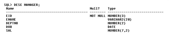
DESC <Table Name>
The ‘DESC’ command helps view the schema of the relation.
DROP TABLE <table name>
This command will drop the table permanently.

🎁 Get the SQL Starter Kit (Free for Students)
Build your SQL foundation with these three essential PDFs:
- SQL Basics Explained
- MySQL Installation Guide
- SQL Practice Questions (20 problems)
This starter kit is free, but requires a quick signup so we can send the PDFs directly to your inbox.
👉 Sign up and receive the download link instantly
Normalization in DBMS
Designing a database structure without proper planning would cause duplicate data and problem updating the database. This will result in an inconsistent database. The process of normalization is to make an efficient database design that allow faster and efficient access while maintaining the accuracy.
What is Normalization?
Normalization is a database design technique that cuts down data redundancy and eliminates undesirable characteristics like Insertion, Update, and Deletion Anomalies. Normalization rules divide larger tables into smaller tables and attach them using relationships. Normalization in SQL’s objective is to get rid of redundant (repetitive) data and ensure data is stored logically.
Normalization is the process of reducing redundancy from a relation or set of relations. Redundancy in relation may cause insertion, deletion, and update irregularities. So, it helps to minimize the extra in relations Normal forms are used to eliminate or cut down excess in database tables.
Normalization is used for mainly two purposes,
• Eliminating redundant(useless) data.
• Verifying data dependencies make sense that is data is logically stored.
What is a KEY in SQL?
A KEY in SQL is a value used to recognize records in a table uniquely. An SQL KEY is a single column or addition of multiple columns used to uniquely spot rows or tuples in the table. SQL Key is used to point out duplicate information, and it also helps establish a relationship between multiple tables in the database.
Note: Columns in a table that are NOT used to identify a record distinctive are called non-key columns.
What is a Primary Key?
A Primary Key is the minimal set of attributes of a table that has the task of uniquely identifying the rows, or we can say the tuples of the given particular table.
A primary key of a relation is one of the possible candidate keys which the database designer thinks it’s primary. It may be selected for favorable, performance, and many other reasons. The choice of the possible primary key from the candidate keys depends upon the following conditions. Rules for defining the Primary key are:-
- Two rows can’t have the same primary key value
- It must be for every row to have a primary key value.
- The primary key field cannot be false.
- The value in a primary key column can never be modified or updated if any foreign key refers to that primary key.
Why do we need Primary Key?
Suppose for any identification we need a different feature that makes it special(different) from others. Everyone has a unique specialty that makes us judge and verifies them based on that quality one has in them.
Similarly, for differentiating a table from others and for identifying them we need a special key control that can be used to validate the records of that table and maintain uniqueness, consistency, and completeness.
Also, for joining any two tables in the relative database systems, a Primary key and another table’s Primary key are known as a Foreign Key, which plays an important role.
So, we can use this Primary Key while creating a table or change it in the database. If a Primary Key is already present in the table, then the server or system will not allow inserting a row with the same key. It helps to improve the security of database records.
What is the Foreign Key?
FOREIGN KEY is a column that creates a relationship between two tables. The purpose of Foreign keys is to maintain data constancy and allow navigation between two different instances of an organization. It acts as a double verification between two tables as it references the primary key of another table.
Foreign Key references the primary key of another Table! It helps connect your Tables
• A foreign key can have a different name from its primary key
• It ensures rows in one table have relative rows in another, Unlike the Primary key, they do not have to be special from others. Most often they don’t have.
• Foreign keys can be invalid even though primary keys cannot be empty.
Example of Foreign Key
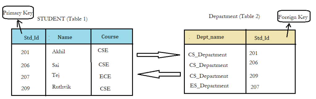
Consider two tables Student and Department having their particular attributes as shown in the below table structure: –
In the tables, one attribute, you can see, is common, that is Std_Id, but it has different key constraints for both tables. In the Student table, the field Std_Id is a primary key because it is uniquely identifying all other fields of the Student table.
On the other hand, Std_Id is a foreign key attribute for the Department table because it is acting as a primary key attribute for the Student table. It means that both the Student and Department table are linked with one another because of the Std_Id attribute.
Difference Between Primary key & Foreign key
Following are the main difference between the primary key and foreign key:
Primary Key
- Helps you to uniquely identify a record in the table.
- Primary Key never accepts clear values.
- The primary key is a clustered index and data in the DBMS table are physically organized in the sequence of the clustered index.
- You can have the single Primary key in a table.
Foreign Key
- It is a field in the table that is the primary key of another table.
- A foreign key may accept multiple empty values.
- A foreign key cannot automatically create an index, grouped or non-grouped. However, you can manually create an index on the foreign key.
- You can have multiple foreign keys on a table.
What is the Composite key?
COMPOSITE KEY is a combination of two or more columns that uniquely identify rows in a table. The combination of columns ensures uniqueness, though individually uniqueness is not guaranteed. Hence, they are combined to uniquely identify records in a table.
The difference between the compound and the composite key is that any part of the compound key can be a foreign key, but the composite key may or maybe not be a part of the foreign key.
What is a Candidate’s Key?
CANDIDATE KEY in SQL is a set of attributes that uniquely identify substrings in a table. Candidate Key is a super key with no repeated attributes. The Primary key should be selected from the candidate keys. Every table must have at least a single candidate key. A table can have multiple candidate keys but only a single primary key.
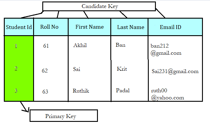
Advantages of Normalization:
- Normalization helps to cut down the data redundancy.
- Greater overall database organization.
- Data consistency within the database.
- Much more workable database design.
- Applies the concept of relational integrity.
Disadvantages of Normalization:
- You cannot start building the database before knowing what the user needs.
- The performance degrades when normalizing the relations to higher normal forms, that is 4NF, 5NF.
- It is very time-consuming and difficult to normalize relations of a peak degree.
- Careless decomposition may lead to a bad database design, leading to serious problems.
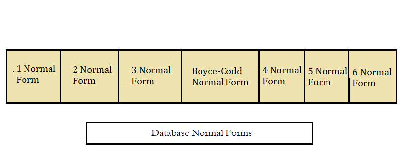
Database Normal Forms
Here is a list of Normal Forms in SQL:
- 1NF (First Normal Form)
- 2NF (Second Normal Form)
- 3NF (Third Normal Form)
- BCNF (Boyce-Codd Normal Form)
- 4NF (Fourth Normal Form)
- 5NF (Fifth Normal Form)
- 6NF (Sixth Normal Form)
1st Normal Form (1NF)
It is Step 1 in the Normalization procedure and is considered the most basic requirement for getting started with the data tables in the database. If a table in a database is not capable of forming a 1NF, then the database design is considered to be poor. 1NF proposes a scalable table design that can be extended easily to make the data retrieval process much simpler.
For a table in its 1NF,
- Data Atomicity is maintained. The data present in each attribute of a table cannot contain more than one value.
- For each set of related data, a table is created and the data set value in each is identified by a primary key applicable to the data set.
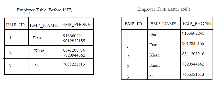
The multiple values from EMP_PHONE made atomic based on the EMP_ID to satisfy the 1NF rules.
2nd Normal Form (2NF)
The basic prerequisite for 2NF is:
- The table should be in its 1NF,
- The table should not have any partial dependencies
Partial Dependency: It is a type of functional dependency that occurs when non-prime attributes are partially dependent on part of Candidate keys.
Example:
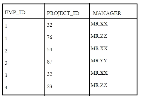
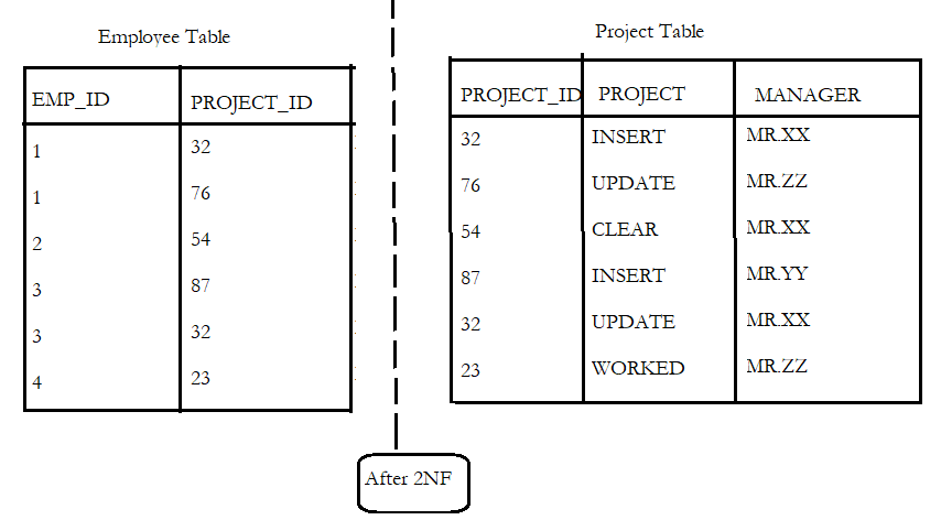
- If manager details are to be fetched for an employee, multiple results are returned when searched with EMP_ID, to fetch one result, EMP_ID and PROJECT_ID together are considered as the Candidate Keys.
- Here the manager depends on PROJECT_ID and not on EMP_ID, this creates a partial dependency.
- There are multiple ways to get rid of this partial dependency and cut off the table to its 2nd normal form, one similar method is adding the Manager information to the project table as shown below.
3rd Normal Form (3NF)
3NF ensures referential integrity, cut down the duplication of data, cuts down data anomalies, and makes the data model more informative. The basic prerequisite for 3NF is,
1. The table should be in its 2NF, and
2. The table should not have any transitive dependencies
Transitive dependency: It occurs due to a resulting relationship within the attributes when a non-prime attribute has a functional dependency on a prime attribute.
Example:
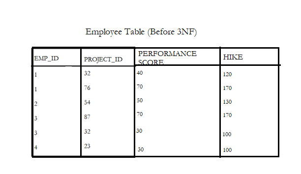
- In Table the PERFORMANCE_SCORE depends on both the employee and the project that he is associated with, but in the last column, HIKE depends on PERFORMANCE_SCORE.
- The hike changes with performance and here the attribute performance score is not a primary key. This forms a transitive dependency
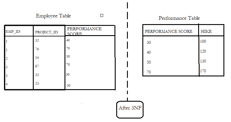
- To get rid of the transitive dependency created, and to satisfy the 3NF, the table is broken as illustrated below:-
Boyce-Codd Normal Form BCNF
BCNF deals with the anomalies that 3 NF fails to address. For a table to be in BCNF, it should satisfy two conditions:
1. The table should be in its 3 NF form
2. For any dependency, A à B, A should be a super key i.e. A cannot be a non-prime attribute when B is a prime attribute.
Example:
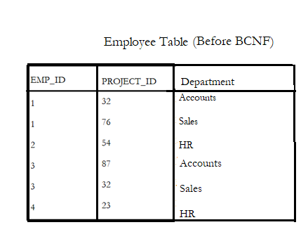
The EMP_ID and PROJECT_ID together can fetch the Department details associated with the employee. i.e.
- EMP_ID + PROJECT_ID → DEPARTMENT
- (Candidate keys)
- DEPARTMENT which is not a super key is dependent only on PROJECT_ID but not dependent on EMP_ID
- Department → Project_ID
- (Non-prime attribute) (prime attribute)
To make this table satisfy BCNF, we need to break the table as shown below:-
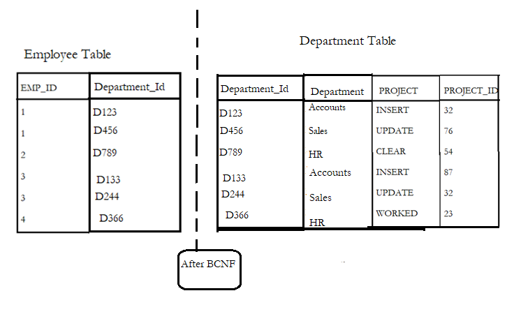
Here the department table is created such that each department id is unique to the department and project-related to it.
It is very important to ensure that the data stored in the database is meaningful and the chances of anomalies are minimal to zero. Normalization helps in reducing data redundancy and helps make the data more meaningful.
Normalization follows the principle of ‘Divide and Rule’ wherein the tables are divided until a point where the data present in them makes actual sense. It is also important to note that normalization does not fully get rid of the data redundancy rather its goal is to minimize the data redundancy and the problems associated with it.
Summary
So, you have learnt the normalization process for designing an efficient database. In most of the cases, the 3rd normal form is enough to create an excellent structure and we never goes to a higher normal form.
It is because of the normal forms a proper functional dependency is maintained.