C Quiz – 2
[HDquiz quiz = “812”]
C Quiz – 1
[HDquiz quiz = “794”]
Program for Sum of First N Natural Numbers
The program adds first N natural numbers (starts from 1) and prints the sum in the console.
We recommend that you try this on your own first and then compare the solutions.
Problem Definition
Natural numbers are all positive numbers greater than number 0 and it does not include the number zero.
For example
Natural\hspace{2mm} numbers = 1, 2, 3, 4, 5, \cdotsThe program reads the value of number N which is a natural number and then sum all other natural numbers up to number N start from 1. Suppose N = 10 then
Sum = 1 + 2 + 3 + 4 + 5 + 6 + 7 + 8 + 9 + 10 = 55
Flowchart – Sum of First N Natural Numbers
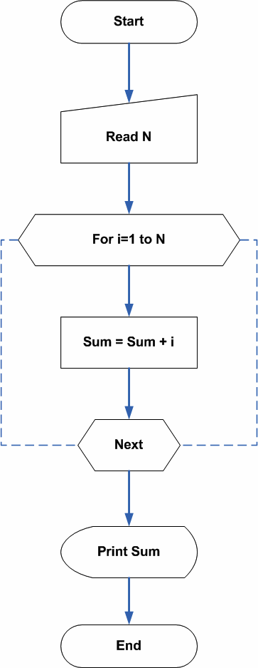
Program Codes – Sum of First N Natural Numbers
/* Program for sum of First N Natural Numbers */
#include <stdio.h>
#include <stdlib.h>
main() {
int num,i,sum;
    sum = 0; /* read the number */
    printf("Enter number to sum:");
    scanf("%d",&num);
    for(i=1;i<=num;i++)     {
    sum = sum + i;
}
printf("sum of %d number is %d\n",num,sum);
    getch();
    return 0;
}
/* Program for sum of First N Natural Numbers */
#include <iostream>
using namespace std;
int main() {
int num, sum = 0;
cout << "Enter number to sum:";
cin >> num;
for (int i = 1; i <= num; i++) {
sum += i;
}
cout << "sum of " << num << " number is " << sum << endl;
return 0;
}/* Program for sum of First N Natural Numbers */
import java.util.Scanner;
public class SumOfN {
public static void main(String[] args) {
int num, sum = 0;
Scanner sc = new Scanner(System.in);
System.out.print("Enter number to sum:");
num = sc.nextInt();
for (int i = 1; i <= num; i++) {
sum += i;
}
System.out.println("sum of " + num + " number is " + sum);
sc.close();
}
}# Program for sum of First N Natural Numbers
num = int(input("Enter number to sum:"))
sum = 0
for i in range(1, num + 1):
sum += i
print(f"sum of {num} number is {sum}")The most important piece of code in the above example is the for loop.
for ( i = 1; i <= num; i++)
{
    sum = sum + 1;
}
The for loop starts from 1 and goes through each digit between 1 and num because variable i is incremented with each iteration ( i++). The value of num is user input and it can be a large number.
The value of i is added to variable sum using the following statement. The value of sum also increments with each iteration of the variable i in the for loop.
sum = sum + i;The final value of the sum is printed as output.
Output
How many numbers to add?:10

sum of 10 number is 55
JavaScript – for Loop
The “For Loop” is the most popular loop in many popular programming languages.
A “For loop” executes a given statement repeatedly until the given condition in the loop becomes false. The loop consists of one or more statements. As long as the condition is “true”, it will execute the statements.
It’s easier to understand this with an example.
We have a web page in the following example, that repeats a given statement using “for loop”. The code prints value of i until the value of i is equal to or greater than 5.
JavaScript Code
var i=0;
for(i=0;i<=5;i++)
{
    document.write("<h3>" + "The Number is"+ i + "</h3>");
 }
The code is added to HTML page called the loop1.html as an internal JavaScript.
Format of the “For loop“
The syntax of “For loop” is simple.
for(i = 0; i <= 5; i++)
{
}
[kate]i[/katex] is loop variable and it could be any lowercase alphabet.
i <= 5 is the loop condition. As long as it is true, the statement inside the loop is executed iteratively.
i++ increments the loop by a count of 1.
Now, we will see how “For loop” works with an example.
HTML Code – loop1.html
<!DOCTYPE html>
<html>
<head>
  <title>For Loop</title>
  <meta charset = "utf-8">
 </head>
 <body>
 <script>
var i=0;
for(i=0;i<=5;i++)
{
    document.write("<h3>" + "The Number is"+ i + "</h3>");
 }
</script>
<p>THIS IS TEST USING INTERNAL JAVA SCRIPT</p>
<p>When you open this web page in a browser that understands the JavaScript, then you will get the following output.</p>

 </body>
 </html>
Make sure that you put the JavaScript code between the <script> … </script> tags. The code can reside in head section or body section. It will still work.
Output – loop1.html
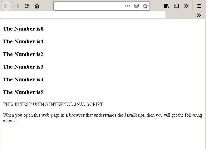
One the HTML page loop1.html is loaded, will print numbers when the “For loop” is executed.
Note how loop is incrementing the numbers by a value of 1. At each iteration of loop, we are incrementing the count by 1 using i++.
JavaScript – Exercise 04 -External JavaScript Files
There are many ways to insert JavaScript into an HTML document. One way is to add the script directly to the HTML document.This method is called adding an “Inline script”.
You can add an inline script at any place within an HTML document, but most web developers like to place the scripts in three locations.
- Head
- Body
- Footer
You have already seen examples of online scripts in exercise 1, exercise 2 and exercise 3.
There is another way to add a JavaScript to an HTML document which is adding an external JavaScript file reference to the HTML page. To help you understand this, we will create a JavaScript file and save it as main.js Then create HTML file called ex04.html and link the main.js to ex04.html document.
External JavaScript Document
In this section, you will create a JavaScript file called main.js file and save it to a folder on your desktop.
Step 1: Create a folder called Exercise 04 on your Windows desktop.
Step 2: Open the folder, Exercise 04 and create a text file and save it as main.js.
Step 3: Open the file main.js again and insert the following JavaScript and save it again.
function message()
{
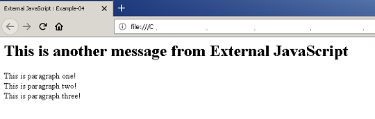
document.write( "<h1>" + "This is another message from External JavaScript" + "</h1>");
document.write("This is paragraph one!");
document.write("This is paragraph two!");
document.write("This is paragraph three!");
}Step 4: Close the file.
Linking JavaScript File to HTML
The next step is to create an HTML file and then link the JavaScript file to the HTML using a reference.
Step 1: Create a new text document called ex04.txt in the Exercise 04 folder on your Windows desktop.
Step 2: Open the text file and insert the following code and save the file as ex04.html in the same location.
Step 3: Link JavaScript file main.js to the ex04.html file using following code.
<html>
<head>
<title>
External JavaScript : Example-04
</title>
</head>
<body onclick="message()">
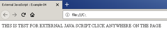
<p> THIS IS TEST FOR EXTERNAL JAVA SCRIPT.</p>
<p>CLICK ANYWHERE ON THE PAGE.</p>
</body>
</html>Step 4: Save and close the file.
The final html page should look like the following.
<html>
<head>
     <title>
        External JavaScript : Example-04
     </title>
     <script type="text/JavaScript" src="main.js">
     </script>
</head>
<body onclick="message()">
     <p>THIS IS TEST FOR EXTERNAL JAVA SCRIPT.</p>
     <p>CLICK ANYWHERE ON THE PAGE.</p>
</body>
</html>
Output to the Browser
To see the output of the HTML and working of external JavaScript, open the HTML file in a browser. You must get the result similar to the following figure, before the onload event. To see this HTML page remove onload = "message ()" from the tag.
You click on the browser window and the following message is printed. If you see the message then external JavaScript is working.
Theory of Computation: alphabet and languages
Fundamental concepts
Symbols
for example:-
1,0, A , a , @ , # are symbols.
Alphabets
Σ = { 0,1 } , Σ = {a,b,c} are examples of alphabet.
Strings or words over Σ
w3= 010 , w4= 0111
Suppose the alphabet is Σ = { a, ε}
w = a ε = ε a = a , where ε is an empty string.
length of string
It is the number of symbols in the string w. The length of empty string is 0.
|ε | = 0
| w| = | a a b a| = 4 ,
It does not matter if the alphabets are repeated.
Concatenation of strings
w7 = 0100111 is concatenation of w3 . w4 .
w1 w2 = ε . b = b . ε = b , where w1 = ε and w2 = b
Finite Automata – I
Formally, “Finite automation is mathematical model of a system with discrete inputs and outputs”. Finite automata describe a system or computer that goes through a fix number of states and has fixed inputs.
For people new to the topic, it is easier to understand using an example.
| States and Symbol |
In this simple example, P and Q are states and ‘a’ is called input alphabet. From the figure we can see that there is transition from one state to another state on receiving the input ‘a’.
Basic Definitions
- A Finite automation (FA) consists of a finite set of states and a set of transitions from state to state that occur on a input symbols chosen from an alphabet ∑.
- For each input symbol there is exactly one transition out to another state.
- q0 is the initial state. There is a state from which automation start all the transitions.
- Some states are accepting states or Final states.
FA is denoted by 5-tuple ( Q, ∑, δ, q0, F ⊂) Q -> Finite number of States ( q0,q1,q2,q3). ∑ -> Finite number of symbols (a,b,c,d,e). δ -> Transition Function ( δ,a). q0 ->Initial State. F -> Final States (F⊆Q) where Q is finite number of states. |
Example of Finite Automata
Consider an finite automata that accepts even numbers binary equivalent.
meaning , 10 in binary is 1010.
At q0 both 0 and 1 are even because they are 0, so q0 is accepting state. Now the automata must read the 1010 which is equal to Ten.
Step 1:
At First it received 1 and transition to q1
Step 2:
Then we received 0 and transition to q3
Step 3:
Then we received a 1 and transition to q2.
Step 4:
Finally, we received a 0, and goes to q0 with is an accepting state.
Now, consider another example, automata reads 1100 which is decimal 12.
Step 1:
First automata reads a 1, and automata goes to q1.
Step 2:
At q1, automata gets another 1 and goes back to q0 which is accepting state.
Step 3:
At q0, receives a 0 and goes to q2 state.
Step 4:
Finally, automata receives a 0 and goes to q0 final state.
Transition Function
A transition function is defined as δ (q, a).
Here q is some state and reads symbol ‘a’, then enters δ (q, a) and moves to next state in automata.
If the next state is an accepting state entire string is accepted successfully.
Steps In Data Cleaning
In the previous article, you have learned about dirty data and issues with data cleaning. Keeping that in mind, we introduce steps in data cleaning.
The data cleaning steps involve data analysis , creating and applying transformation rules, and back-flow.
Step 1: Data Analysis
Before you clean the data, you must analyze it using the definition of a dirty data. The data that has no common standards, missing data, duplicate data, factually incorrect, and contains many inconsistencies such as inconsistent associations, semantic inconsistencies, and referential inconsistencies are dirty data.
Therefore, identifying such data is the first step towards cleaning the data set. Also, you must obtain the metadata.
Step 2: Create Transformation Rules
The transformation rules can transform data from its “dirty” form to the required “clean” form. The transformation can be applied either at the schema level or data level.
The schema level transformation is necessary because of poor schema design of the databases and multiple sources of data. Every database has its own schema structure and requires that it must be optimized.
The data set may also has missing and duplicate data, and incorrect aggregated values. Therefore, the transformation rule for both schema and data level depends on the source of data. Is the data from single source or multiple sources ?
Step 3: Rule Verification
Once the rules are in place, you must verify that it works by applying it on test data sets.
Step 4: Transformation
Once you are satisfied with the test results, apply the transformation rules on the actual data set.
Step 5: Backflow
Re-populate the data sources with cleaned data is called back-flow.
Data Analysis Techniques
There are many data analysis techniques used to find dirtiness in the data. See the table below.
| Problems To Be Detected | Meta-data Used |
| Illegal values | (max, min), (mean, deviation), cardinality |
| Spelling Mistakes | Hashing, N-gram outliers |
| Lack of Standards | Column comparison ( compare value sets from given column across tables ) |
| Duplicate and Missing Values | Compare cardinality with rows, detect nulls, use rules to predict incorrect or missing values. |
In the next article, we will discuss about transformation algorithms that remove the dirtiness of data.
JavaScript References
In this document you will find JavaScript references for all object classes.
String Functions
- JS: repeat()
- JS: endsWith()
- JS: split()
- JS: substring()
- JS: toUpperCase()
- JS: toLowerCase()
- JS: indexOf()
- JS: lastIndexOf()
- JS: join()
Array Functions
R Basics
In this article, you will learn about basics building blocks of R programming such as constants, variables and vectors.
R programming uses various arithmetic operators to manipulate constants, variables and vectors.
Arithmetic operators in R
In R programming, the following are the arithmetic operators.
| Operator | Meaning |
| + | addition |
| – | subtraction |
| * | multiplication |
| / | division |
| ^ | exponential |
| %% | mod |
Apart from the above the R programming also use some math functions such as sqrt() and abs(). The sqrt() function returns square root of a number or vector and the abs() function gives absolute value of a variable or vector.
Constants in R
The constant is a number, or character that can be manipulated without assigning it a name. You can use R console like a calculator simply using the constants.
Consider following examples.
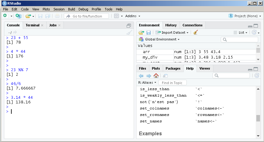
From the above figure, it is clear that you can use the R console as calculator. Simply type the operators and operands and you get the output. Note that this only works for numeric data.
Joining two strings would result in error.
> "Hello" + "World"
Error in "Hello" + "World" : non-numeric argument to binary operator
>
Note: If you want to clear the console press Ctrl + L on your keyboard.
Variables in R
Variables are used to store values that are used in expressions. The results of expressions are also stored in variables.
Variables can store different types of data such as numbers, strings, and vectors.
In R programming, you have to assign values to variables. In case, you are using R console then the traditional assignment operator (=) works with new assignment operators given below.
| Assignment Operator | Meaning |
| <-, <<-, = | Right to left assignment |
| ->, ->> | Left to right assignment |
Following are some examples of right to left variable assignment in R.
## Right to Left assignment
> A = 200
> A
[1] 200
>
> B <- 300
> B
[1] 300
>
> C <<- 400
Error: cannot change value of locked binding for 'C'
> B <<- 400
> B
[1] 400
> D <<- 500
In the example, the C <<- 400 failed because <- and <<- works differently. The operator <– means “assign the left hand value to right hand variable”, however, C <<- 400 means “find the variable C in the current scope and then if found assign the value of 400” .
The variable C <<- 400 is not working because C is not defined earlier. But, B <<- 500 works as it is available in the current scope.
Let us see some more examples right to left of assignment
> 100 -> P
> P
[1] 100
> 200 ->> Q
> Q
[1] 200
>
Vectors in R
You can create vectors in R programming. These vectors can take many types of data such as strings, numbers, double, Boolean, etc.
To create a vector use following syntax.
>  my_vector <- c(1,2,4,5, 34.2, "Hello", TRUE)
> my_vector
[1] "1"     "2"     "4"     "5"     "34.2"  "Hello" "TRUE"
>
You can perform arithmetic operations with a vector like any ordinary variable. Consider the following example.
> c(20, 30, 50) * 5
[1] 100 150 250
>
In the example above, the number 5 is multiplied with each element of the vector.
Similarly, you can append an array with more elements.
> myVector <- c(27, 55, 33.2)
> z <- c(myVector, 100, 200)
> z
[1]  27.0  55.0  33.2 100.0 200.0
>
Using the above technique we have added two more elements 100 and 200 to the existing vector.
Arithmetic Between Two Vectors
You can even perform arithmetic operation between two vectors. Here is an example.
> a_vector <- c(100, 200, 300, 400) / c(2, 4, 6, 8)
> a_vector
[1] 50 50 50 50
Each element of the first vector is divided by the corresponding element of the second vector. Therefore, 100/2, 200/4, 300/6 and 400/8 give the output of 50 50 50 50.
What if the second vector is smaller than the first one ?
> result_vector <- c(12, 44, 66, 22)/ c(2, 3)
> result_vector
[1]  6.000000 14.666667 33.000000  7.333333
>
If the second vector is smaller than the R programming “recycles” the second vector against the first vector. In the example above, 12/2, 44/2, 66/2 , and 22/3 resulted in 6.000000 14.666667 33.000000 7.333333.Note how second vector repeat itself for the division.
If the second vector elements does not cover all elements in the recycling process, then the arithmetic operation will fail.
> c_vector <- c( 122, 45, 55) * c(23, 44)
Warning message:
In c(122, 45, 55) * c(23, 44) :
  longer object length is not a multiple of shorter object length
>
The error message clearly says that the shorter array must be multiple of longer vector for recycling to happen.