Engineering Math Archives - Page 2 of 3

Composite Functions

In this article, we you will learn about composite functions, it means that a function can become input of another function. Before you learn about the composite functions, you must be familiar with the arithmetic of functions which means given two function , you will be able to perform basic arithmetic operations on the function itself. Identifying Domain

Sometimes the function expression is given, but domain is not specified. In such cases, you must identify the domain of given function. Suppose

$\begin{align*} f(x) = x^2 -1\end{align}$

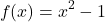
is a function whose domain is $D_f$ which is “all real numbers”, because the function is true for all real numbers. Another function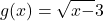

$\begin{align*} g(x) = \sqrt{x - }3\end{align}$

has a domain $D_g$ which must have all numbers that are $x - 3 \geq 0$ otherwise the function is invalid. Therefore, $D_g$ contains all numbers in the interval $[3, -\infty]$ .

Why this is important ? because when we perform arithmetic operations on two or more functions the domain of new function is set of all real numbers that belong to both $D_f$ and $D_g$ , that is, $(D_f \cap D_g)$ .

Arithmetic Operations on Functions

Normal arithmetic operations are possible on functions too. If $f$ and $g$ are two functions, then there are four operations possible on these functions.

Sum $(f + g)$
Difference $(f - g)$
Product $(fg)$
Quotient $(\frac{f}{g})$

Now we discuss about each of these operations.

Sum of functions

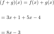
The sum of functions is

$\begin{align*}(f + g)(x) = f(x) + g(x)\end{align}$

The expressions of both functions are added together to form a new function. For example, if $f(x) = 3x +1$ and $g(x) = 5x - 4$ , then

$\begin{align*}\\&(f + g)(x) = f(x) + g(x)\\ \\ & = 3x + 1 + 5x - 4\\ \\&=8x - 3\end{align}$

Difference of functions

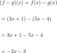
The difference of functions is

$\begin{align*}(f + g)(x) = f(x) - g(x)\end{align}$

The expressions of function $g$ is subtracted from expression of function $f$ to form a new expression for $f-g$ . For example, if $f(x) = 3x +1$ and $g(x) = 5x - 4$ , then

$\begin{align*}\\&(f - g)(x) = f(x) - g(x)\\ \\ & = (3x + 1) - (5x - 4)\\ \\ & = 3x + 1 - 5x - 4 \\ \\&=-2x -3 \end{align}$

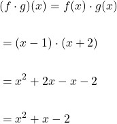
Product of functions

The product of the functions is

$\begin{align*}(f \cdot g)(x) = f(x) \cdot g(x)\end{align}$

The expressions of function $f$ and $g$ is multiplied to get the new product expression of $f \cdot g$ . Each term is of $f$ is multiplied with each term of $g$ . For example, if $f(x) = x - 1$ and $g(x) = x +2$ are two expressions, then

$\begin{align*}\\&(f \cdot g)(x) = f(x) \cdot g(x)\\ \\ & = (x - 1) \cdot (x + 2)\\ \\ & = x^2 + 2x -x -2\\ \\&=x^2 + x -2\end{align}$

Quotient of functions

The quotient of functions is obtained by dividing two functions, which is

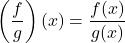
$\begin{align*}\left(\frac{f}{g}\right)(x) = \frac{f(x)}{g(x)}\end{align}$

The functions are divided to get the quotient, however, there is one condition, that is, $g(x) \ne 0$ , otherwise the quotient of function will be “divide by 0” which is “undefined“.

Therefore, if $f(x) = x^2 + x - 2$ and $g(x) = x + 2$ , then

$\begin{align*}\\&\left(\frac{f}{g}\right)(x) = \frac{f(x)}{g(x)}\\ \\ & = \frac{x^2 + x -2}{x + 2}\\ \\ & Factor \hspace{2mm} the \hspace{2mm} numerator \\ \\ &=\frac{ (x-1)(x+2)}{x+2}\\ \\&=x - 1\end{align}$

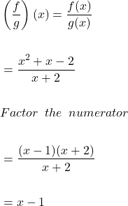
The domain of $(f + g)$ , $(f - g)$ , $(fg)$ is set of all reals numbers that are common to domain of $f(x)$ and $g(x)$ which is $(D_f \cap D_g)$ except where $g(x) \ne 0$ for $(\frac{f}{g}$ .

Composite Functions

The composite functions or the idea of composition of functions is simple. Suppose there are two functions, $f$ and $g$ , then if function $g$ becomes input for function $f$ , it is called “composition of function $f$ with function $g$ or simply a composite function.

Let us try to understand this with an example, suppose Nancy work as a maid, and get paid $x$ amount every week and after paying taxes she receives only $80%$ of her earnings. Each week she spends $\textdollar 50$ for grocery from her earning . The total earning of Nancy after paying taxes can be defined by function $g(x) = 0.80 \cdot x$ . Her savings after expense of $\textdollar50$ can be defined as function $f(x) = x - 50$ .

$\begin{align*}Each \hspace{2mm} week \hspace{2mm} Nancy's \hspace{2mm} saving = (f \circ g)(x) = f(g(x))\\ \\ f(0.80x) = 0.80x - 50\end{align}$

If her gross earning is $\textdollar 200$ , then her saving would be

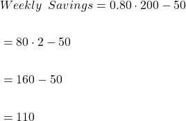
$\begin{align*}&Weekly \hspace{2mm} Savings = 0.80 \cdot 200 - 50\\ \\&= 80 \cdot 2 - 50 \\ \\&=160 - 50\\ \\ &= 110 \end{align}$

Therefore, total saving after paying taxes and expenses of $\textdollar 50$ is $\textdollar 110$ .

What is the domain of a composite function?

If $(f \circ g)(x)$ is a composite function such that $(f \circ g)(x) = f(g(x))$ . Then the domain of composite function must be

$x \in D_g$ meaning “ $x$ must be in the domain of $g(x)$ .
$g(x) \in D_f$ meaning “ $g(x)$ must be in the domain of $f(x)$ .

Therefore, while finding the domain of a composite function, we must first exclude all values of $x$ than can make the function $g(x)$ “invalid”. Also, if $x$ happens to be valid, that is, $x \in D_g$ , then $g(x)$ must be valid value for the function $f(x)$ . If $g(x)$ happens to invalid value, then both $g(x)$ and $x$ must be excluded from the domain of composite function $(D_g \cap D_f)$ .

Decomposing Functions

Like composing two functions, it is possible to decompose a function because we know that “composition of two functions” creates a new function. Consider the following example,

$\begin{align*}h(x) = \sqrt{x - 1}\end{align}$

Here we can clearly see that there are two functions involved in the expression. Therefore, $h(x) = \sqrt{x -1} = \sqrt{c}$ where $c = x -1$ which implies that $c = g(x) = x -1$ .

We can write the function $h(x)$ and $g(x)$ as composition of function $h \circ g$ where $h(x) = \sqrt{x}$ and $g(x) = x -1$ .

post

Transformation of Graphs

Graph of function does not remain the same. It changes its shape or position when values are added, subtracted or multiplied by the equation of the graph. This kind of change in the graph is called a transformation of the graph of functions.

You must be familiar with the transformation happens to a graph of function once the equation changes. You should be able to tell the changes in the graph by looking at the new graph of the equation.

Before you begin, learn about graph and graphs of equations, functions, a graph of functions. If you know them already skip ahead and continue reading.

Types of Graph Transformation

The graph transformation is broadly classified into two types.

Transformation of Position
Reflection
Transformation of the shape of Graph

We shall discuss each of these transformations in more detail in coming sections.

Transformation of Position

This type of transformation changes the position of the original graph to left, right, top and bottom by a few units. The graph is no longer in its original position.

If $y = f(x)$ is a function and $c$ is a positive real number, then shift in the graph position is represented as

Shift of c units upward (y-axis) : $g(x) = f(x) + c$

Shift of c units downward (y-axis) : $g(x) = f(x) - c$

Shift of c units left (x-axis) : $g(x) = f(x + c)$

Shift of c units right (x-axis) : $g(x) = f(x - c)$

To understand the positional shift in graph, check the examples in following sections.

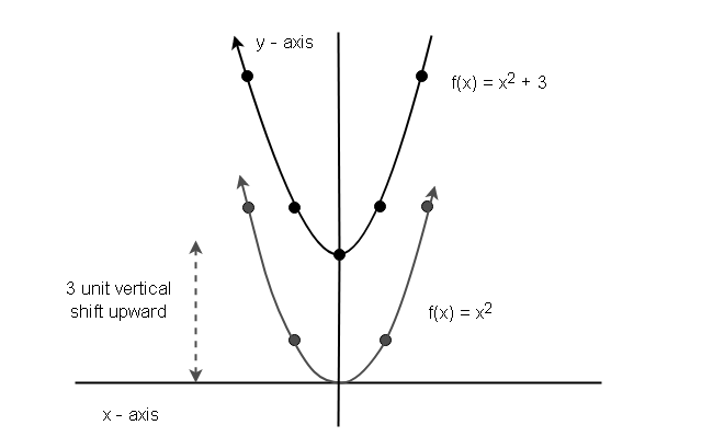
Example 1:

Let $f(x) = x^2$ and $c = 3$ . Then the function $h(x)$ is given as follows.

h(x) = f(x) + c

substituting value $f(x)$ and $c$ , we get

h(x) = x^2 + 3

Create a table of values for $(x, h(x))$ to plot the graph of the function.

x	h(x)
-2	7
-1	4
0	3
1	4
2	7

Using the above value plot a graph of function for $h(x) = x^2 + 3$ .

Figure 1 – Transformation of Function_ x^2 + 3

Example 2:

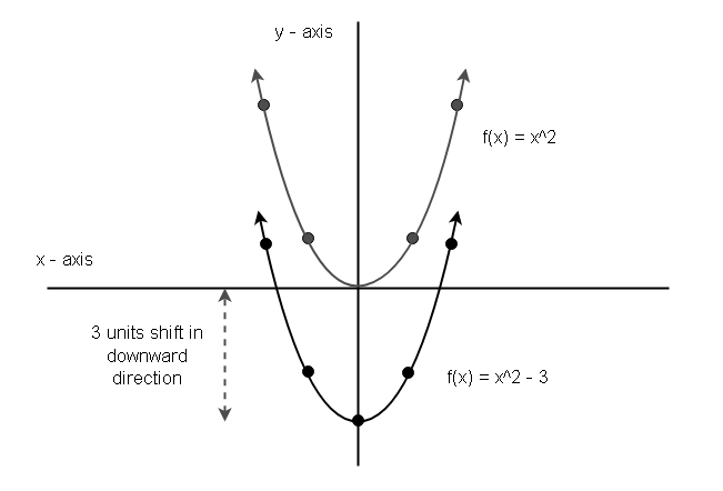
Now, we plot the graph of $h(x) = f(x) - c$ .

Substituting for $f(x)$ and $c$ , we get.

h(x) = x^2 - 3

Once, again create a table with values for $(x, h(x))$ .

x	h(x)
-2	1
-1	-2
0	-3
1	-2
2	1

You can plot a graph using the above table.

Figure 2 – Transformation of Graph_ x ^2 – 3

Example 3:

The horizontal shift in a graph of a function is different from vertical shift because the value of a range is unaffected, but the value of domain x is increased or decreased. Thus causing right or left shift horizontally.

Suppose $f(x) = x^2$ be the function and $c = 3$ be the positive real constant. Then

$h(x) = f(x-c)$ implies $h(x) = (x - c)^2$

In other words, value of $x$ in $h(x)$ is reduced by $c$ units in $f(x)$ to get the output.

\begin{aligned} &h(5) = f(5 - 3)\\\\ &= (5 - 3)^2\\\\ &= 2^2\\\\ &= 4 \end{aligned}

Let us now plot the graph of function $h(x)$ .

x	f(x – 3)	h(x)
3	f(0)	0
2	f(-1)	1
4	f(1)	1
1	f(-2)	4
5	f(2)	4

The graph of function $h(x)$ look like the following.

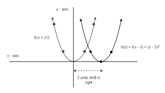
Figure 3 – Transformation of Graph_ f(x – 3)

Clearly, the graph shifted to 3 units right horizontally.

Example 4:

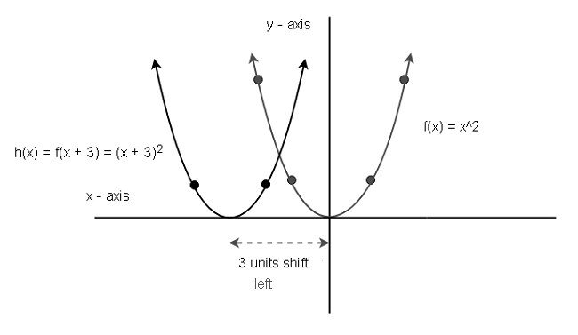
The left shift transformation is similar to the right shift. Let $h(x) = f(x + c)$ . The function $f(x) = x^2$ and $c = 3$ .

The graph of this function will look like the following. The procedure to plot the graph is similar to the right shift transformation.

Figure 4 – Transformation of Graph_ f(x + 3)

Combining More Than one Shift

It is possible to combine two or more shifts. Consider the following functions.

\begin{aligned} &f(x) = x^2\\\\ &g(x) = f(x - 3) = (x - 3)^2\\\\ &h(x) = g(x) + 1 \end{aligned}

It implies that

h(x) = (x - 3)^2 + 1

Therefore, the graph will shift 3 units right horizontally and shift 1 unit up vertically.

Reflection of a Graph

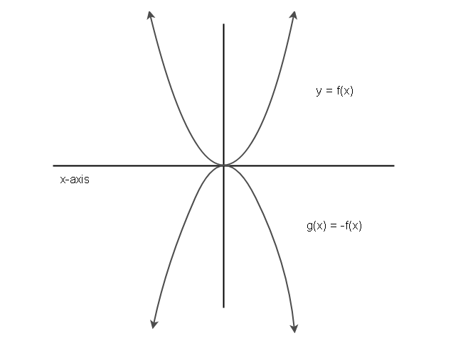
Reflection is another type of graph transformation. It does not change position but uses the x-axis or y-axis to reflect a graph of a function.

Reflection on x-axis: $g(x) = -f(x)$

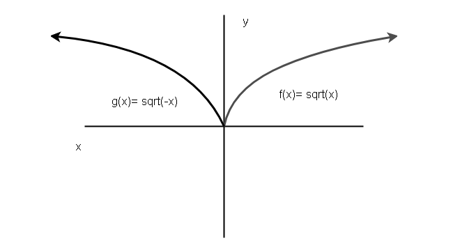
Reflection on y-axis: $g(x) = f(-x)$

Let us see few examples to find out what reflection of a graph means.

Example 5:

Let $f(x) = x^2$ be the original equation. If $-f(x)$ represents the reflection of the function $f(x)$ on x-axis, then the graph will look like below diagram.

Figure 5 – Reflection on X-axis

Example 6:

Let us take another example for reflection along y-axis. The function $f(-x) = \sqrt -x$ is reflection of $f(x) = \sqrt x$ .

For this example, we will plot the graph of both $f(x)$ and $f(-x)$ .

Figure 6 – Reflection on y-axis

Transformation of the Shape of Graph

The transformation of position or the reflection does not change the shape of the graph itself. It just moves the graph to a different location in the coordinate system. If $y = f(x)$ is the graph of function then transformation is represented by $g(x) = cf(x)$ , where it is a vertical stretch if $c > 1$ and vertical shrink if $0 < c < 1$ .

If $y = f(x)$ is the graph of function then its transformation is $g(x) = f(cx)$ , where it is a horizontal shrink if $c > 1$ and horizontal stretch if $0 < c < 1$ .

Example 7:

To understand the vertical transformation of shape, consider an example. Let $f(x) = |x|$ be a function and $c$ be a real constant.

You have two cases, case 1 when $c > 1$ and case 2 with $0 < c < 1$ . Suppose $c = 2$ then

$g(x) = 2|x|$ , we know that this is case 1 and result in a vertical stretch.

Find all the points to plot the graph of function $g(x)$ .

x	f(x) = \|x\|	g(x) = 2\|x\|
0	0	0
1	1	2
2	2	4
3	3	6
4	4	8

You can easily plot the graph of function $g(x)$ using the above points, which is given below.

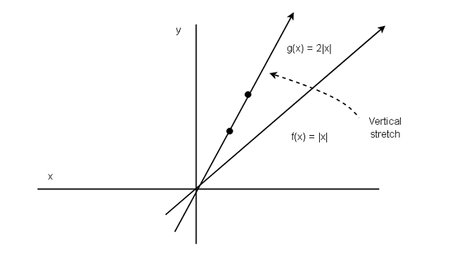
Figure 7 – Transformation of Shape: Vertical Stretch

Suppose $0 < c < 1$ , then its case 2 – vertical shrink. Let us plot the graph of the equation for case 2 when $c = 1/2$ .

x	f(x) = \|x\|	g(x) = 1/2\|x\|
0	0	0
1	1	1/2
2	2	1
3	3	3/2
4	4	2

The graph of the function $g(x) = 1/2|x|$ is given below.

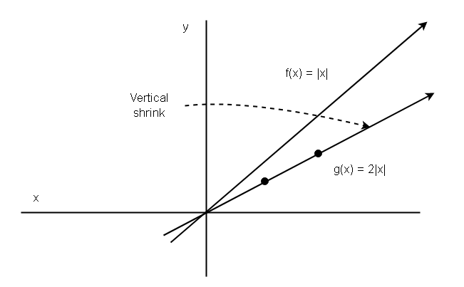
Figure 8 – Transformation of Shape_Vertical Shrink

The graph of function $g(x)$ shows that the vertical shape transformation has happened.

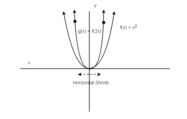
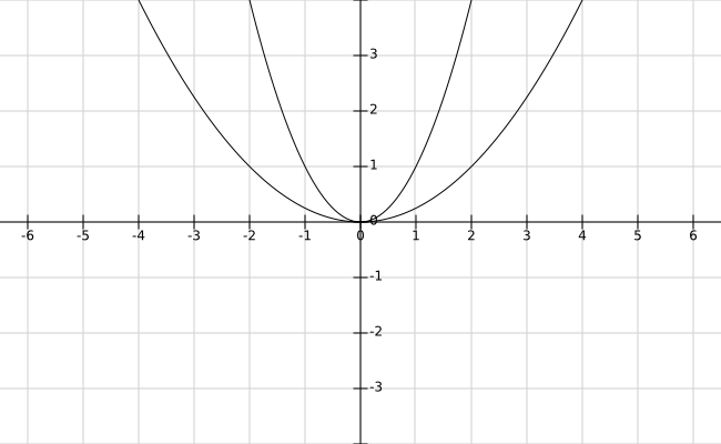
The horizontal shape transformation also happens in the same way. Let $f(x) = x^2$ be the function, and $g(x) = f(cx)$ be the horizontal shrink when $c > 1$ and horizontal stretch when $0 < c < 1$ .

Suppose $c = 2$ for horizontal shrink and $c = 1/2$ for horizontal stretch respectively. Then the graph of function $g(x) = f(cx)$ is given below.

x	f(x) = x^2	g(x) = f(2x), c > 1	g(x) = f(1/2x), 0 < c < 1
2	4	16	1
1	1	4	1/4
0	0	0	0
-1	1	4	1/4
-2	4	16	1

Example 8:

The graph of function g(x) with horizontal shrink.

Figure 9 – Transformation of Shape_Horizontal Shrink

Example 9:

Similarly, we can plot the graph of horizontal stretch.

Figure 10 – Horizontal Stretch

post

Types of Functions and Their Graphs

You can identify a function by looking at its graph. This article, we explore different types of function and their graphs.

Prerequisite to learn from this article is listed below.

There is a relationship between a function and its graph. With the help of a graph of function, you can discover may properties which the algebraic form does not provide.

The graph of functions helps you visualize the function given in algebraic form. By look at an equation you could tell that the graph is going to be an odd or even, increasing or decreasing or even the equation represents a graph at all.

Linear Function
Squaring Function
Cubic Function
Square Root Function
Reciprocal Function
Step Function
Piece-Wise Function

Linear Functions

The linear functions are straight lines. Read the following article to learn more about linear function.

Linear Equations

Squaring Functions

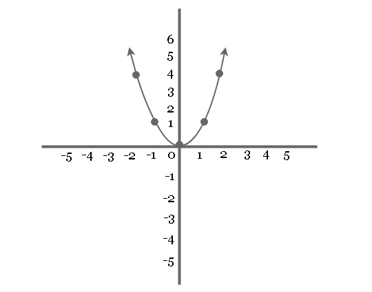
The graph of squaring function is commonly known as a parabola which is a U-shaped curve.The diagram for squaring function $f(x) = x^2$ is given below.

Squaring Functions

Properties of a Squaring Function

The properties of a squaring function are the domain and range, intercepts, etc.

The domain of squaring function set of all real numbers that corresponds to x-axis.
The range of squaring function is all non-negative real numbers because the graph is U-shaped.
The function is an even function because it is symmetric along the y-axis.
The intercept of squaring function is at point (0, 0).
The graph of squaring function has relative minimum at (0, 0).
The squaring function graph is decreasing between interval $(-\infty, 0)$ .
The graph is increasing between the interval $(0, \infty)$ .

Graph of Cubic Function

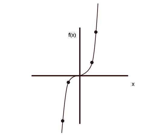
The graph of cubic function is in positive side and negative side unlike squaring function which is only on positive side.

f(x) = x^3

If you plot the graph then it look like the one below. Let us use the following table to plot the graph of cubic function.

x	y = f(x) = x^3	point
-2	-8	(-2, -8)
-1	-1	(-1, -1)
0	0	(0, 0)
1	1	(1, 1)
2	8	(2, 8)

The graph of cubic function look like the following.

Graph of Cubic Function

Properties of Cubic Function

Cubic function has following properties.

The cubic function is an odd function.
The cubic function is symmetric along the origin.
The domain of cubic function is set of all real numbers.
The range of cubic function is set of all real numbers because the function has interval between $(-\infty, \infty)$ .
The intercept of the graph is at (0, 0).
The function is always increasing between the interval – $(-\infty, \infty)$ .

Graph of Square Root Function

A graph of function $f(x)$ where a value of $x$ results in $\sqrt {x}$ .

f(x) = \sqrt{x}

Let us plot the graph of the square root function by obtaining some points. We used calculator to compute some values.

The graph of the squaring function is given below.

Graph of Squaring Function

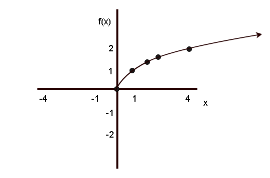
As you can see that the graph is only on positive side for both $x$ and $f(x)$ .

Properties of Squaring Function

The graph of squaring function is given below.

The domain is set of non-negative real numbers $(0, \infty)$ .
The range is is set of non-negative real numbers $(0, \infty)$ .
The intercept of the graph is at $(0, 0)$ .
It is increasing between the interval $(0, \infty)$ .

Graph of Reciprocal Function

Let $f(x)$ be a function, then

f(x) = \frac{1}{x}

is called a reciprocal function.

To plot the graph of reciprocal function, let us find all the points first.

x	f(x) = 1/x	point
-3	-1/3	(-3, -1/3)
-2	-1/2	(-2, -1/2)
-1	-1	(-1, -1)
0	undefined	undefined
1	1	(1, 1)
2	1/2	(2, 1/2)
3	1/3	(3, 1/3)

The graph of reciprocal is shown below.

Graph of Reciprocal Function f(x) = 1/x

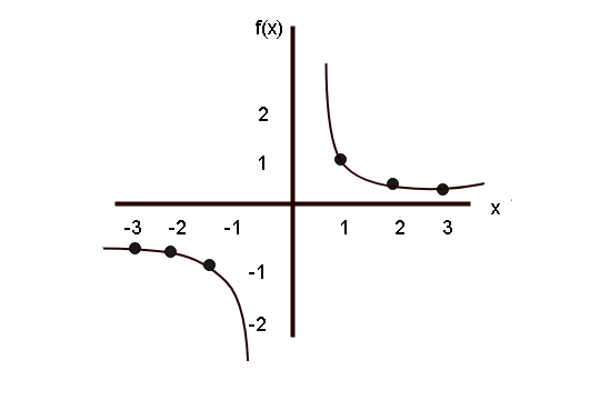
Properties of Graph of Reciprocal Function

The reciprocal function is symmetric along the origin, but it never touches the origin itself. The properties of a reciprocal function is given below.

It is odd function because symmetric with respect to origin.
It has no intercepts.
The domain of reciprocal function is between $(-\infty, 0) \cup (0, \infty)$ .
The range of reciprocal function is $(-\infty, 0) \cup (0, \infty)$ .
It is decreasing in the interval $(-\infty, 0)$ .
and increasing in the interval $(0,\infty)$ .

Graph of Step Function

The graph of step function actually look like a staircase with steps.

Let $f(x) = [[x]] + 1$ , be the step function where

[[x]] mean find the a value ‘greater than or equal to x‘.

We must find points to plot the graph of step function.

x	f(x) = [[x]] + 1	points
-2	-1	(-2, 1)
-1	0	(-1, 0)
0	1	(0, 1)
1	2	(1, 2)
2	3	(2, 3)

The graph of step function is shown below.

Graph of Step Function

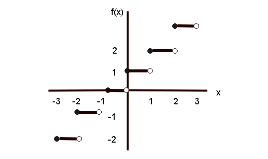
Properties of Step Function

The properties of step function are given below.

Domain is set of all real numbers.
Range of function is set of all integers.
The y-intercept is (0,0) and x-intercept is [0, 1).
The graph is constant between each pair of integers.
The graph jumps vertically one unit for each y-value.

Graph of Piece-wise Function

The graph of piecewise function is already discussed in previous lessons.

Graphs of Functions

If you remember these basic graph of functions used in algebra, then it is easier to learn higher and complex graphs. Later , when you learn calculus, visualizing concepts is much easier with a graph of function.

post

Odd Even Functions

The graph of equation has symmetry along the x-axis or y-axis. In this article, the symmetry of a graph of function is defined in terms of even and odd function.

Prerequisite for this articles is listed below.

Even Function

Let’s understand the even functions first. The function $y = f(x)$ is even function, if for every x in domain of $f$ .

f(-x) = f(x)

For example,

Let $y = f(x)$ be a function where

f(x) = x^2

The function will square any input value for $x$ and output $f(x)$ . Let us put some values for $f(x)$ , see the following table of values.

x	y = f(x)	point
-2	4	(-2, 4)
-1	1	(-1, 1)
0	0	(0, 0)
1	1	(1, 1)
2	4	(2, 4)

The table shows that any $f(-x)$ values is equal to $f(x)$ .

Even Function F(x) = x^2

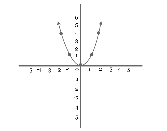
The graph of even function is symmetric along the y-axis.

Odd Functions

The odd function is different from even function in terms of symmetry of graph of the function. The function $y = f(x)$ is odd function if for every $x$ in the domain of $f$ .

f(-x) = -f(x)

Consider the following table of points for the function $y = f(x) = x + 1$ .

x	y = f(x) = x + 1	point
-3	-2	(-3, -2)
-2	-1	(-2, -1)
-1	0	(-1, 0)
0	1	(0, 1)
1	2	(1, 2)
2	3	(2, 3)

The graph of odd function shows that $f(-x) = x + 1$ is $-f(x)$ .

Odd Functions

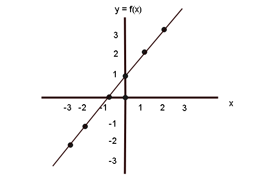
The graph of odd function is symmetric along the y-axis.

post

Increasing, Decreasing and Constant Functions

Previously you learned about functions, graph of functions. In this lesson, you will learn about some function types such as increasing functions, decreasing functions and constant functions. These concepts are explained with examples and graphs of the specific functions where ever necessary.

Increasing, Decreasing and Constant Functions

Functions are increasing, decreasing and constant when you plot the graph of the function in a coordinate system. Let’s define the meaning of these functions.

Increasing function

A function $f(x)$ is increasing in an interval for any $x_1$ and $x_2$

if $x_1 < x_2$
implies $f(x_1) < f(x_2)$

Example:

Let $f(x) = x^2 + 1$ be a function. Find all the values for the function to plot the graph.

x	f(x)	(x, f(x))
-1	2	(-1, 2)
0	1	(0, 1)
1	2	(1, 2)
2	5	(2, 5)

The graph of the function will look like the following.

Figure 1 – Increasing Functions

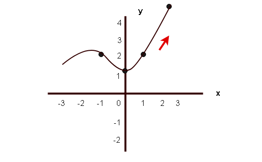
In the above graph, the function is increasing between the interval of (0, 2).

The value of $x_1$ is 0 and $x_2$ is 3,

The value of $f(x_1)$ is 1 and $f(x_2)$ is 5.

Therefore,

$x1 < x2$ implies $f(x_1) < f(x_2)$ is true and it is an increasing function.

Decreasing Function

A function $f(x)$ is decreasing in an interval for any $x_1$ and $x_2$

if $x_1 < x_2$
implies $f(x_1) > f(x_2)$

Example:

Consider a function $f(x) = x^2$ . The function is a parabola. Let’s draw the graph of this function in a Cartesian plane or co-ordinate system.

Before plotting the graph, you need to find points for the graph of the function. A table of points is given below.

x	f(x)	(x, f(x)
-2	4	(-2, 4)
-1	1	(-1, 1)
0	0	(0, 0)
1	1	(1, 1)
2	4	(2, 4)

The graph of the parabola is given below.

Figure 2- Decreasing Functions

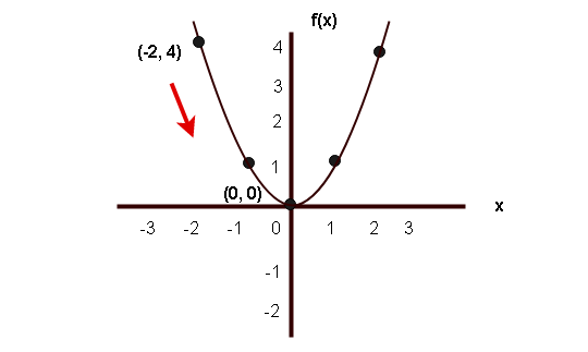
In the above graph, the function is decreasing between the interval ( -2, 0).

The value of $x_1$ is -2 and the value of $x_2$ is 0.

The value of $f(x_1)$ is 4 and the value of $f(x_2)$ is 0.

Then

$x_1 < x_2$ is true and $f(x_1) > f(x_2)$ is also true. Hence, the function is a decreasing function between the interval $(-2, 0)$ .

Constant Function

The function is a constant function in an interval for some $x_1$ and $x_2$

if $x_1 < x_2$
implies $f(x_1) = f(x_2)$

This is simplest form of graph of a function and such a function is always a straight line on the coordinate system.

Let $f(x) = 3$ be the constant function. It means for any value of $x$ in the domain, the value of $f(x)$ is 3.

The graph of constant function is given below.

Figure 3 – Constant Function

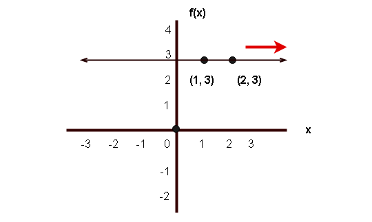
In the above graph of the constant function.

The value of $x_1$ is 1 and the value of $x_2$ is 2.

The value of $f(x_1)$ is 3 and the value of $x_2$ is also 3.

Therefore,

$x_1 < x_2$ and $f(x_1) = f(x_2)$ implies that the function is a constant function.

post

Graphs of Functions

In the previous lesson, you learned about functions and different ways to represent a function. One of the way to represent the function is using graphs. In this lesson, you will explore the graphs of functions and understand how to determine the domain and range of function from its graph. You will learn about vertical line testing and how to find zero of a function.

The graph of a function is the ordered pair $(x, f(x))$ .

x = length along the x-axis.
y = f(x) = length along the y-axis.

Let’s draw the graph of a function and see how it works.

Figure 1 – Graph of a Function (x, f(x))

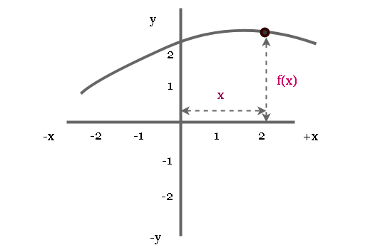
The above diagram clearly shows that the graph has $y = f(x)$ for some input x.

Finding Domain and Range using Graph of Function

You can easily find the domain and range of a function using graph of the function. Plot the graph of the function using algebraic equation of the function.

See the graph below

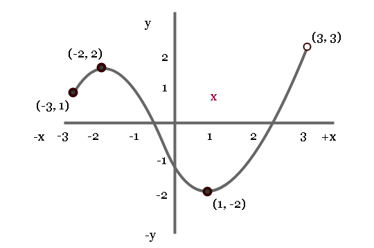
Figure 2 – Finding Domain and Range from Graph

In the graph some points are closed or filled and some of them are not-filled or open.

The points (-3, 1) , (-2, -2) and (1, -2) are in the domain of the function
However, (3, 3) is not defined and not in the domain of the function.

Therefore,

The domain of the function $y = f(x)$ is between the interval [-3, 3). We have taken the left most and right most value of x as the domain. But do not forget to check if the interval is open or closed.

Range of the Function

In the diagram above, the highest point and the lowest point defined are (-2, 2) and (1, -2) respectively. Then the range of the function using graph is the closed interval [2, -2] because both points are defined.

Vertical Line Test for Graph

You can determine whether a graph belongs to a function or not, using a vertical line test.

Vertical Line Test

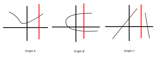
In the above diagram the red line, intersect the graph A at one place. The graph A belongs to a function. The line crosses the graph B at two places. It is not a graph of a function.

The graph sometimes is not defined for some functions and as a result the line will not intersect the graph at all. But this does not mean that it is not a graph of a function, just because it is not defined as in the case of graph C.

Zero of a Function

Previously you learned about the intercepts of an equation. The graph of a function has x-intercept which is (a, 0). The zero of the function is the value of x for which $f(x) = 0$ .

Figure 4 – Zero of a Function

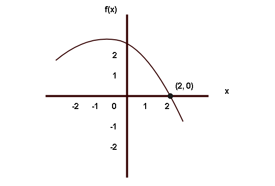
In the graph shown above, the zero of the graph is the point (2, 0) where the graph intersects the x-axis. Some graphs have more than one zero because they intersect the x-axis more than once.

post

Functions

In the previous lesson, you learned about Cartesian coordinate system, graph of equations and linear equations. These are prerequisites to learn about function in this lesson.

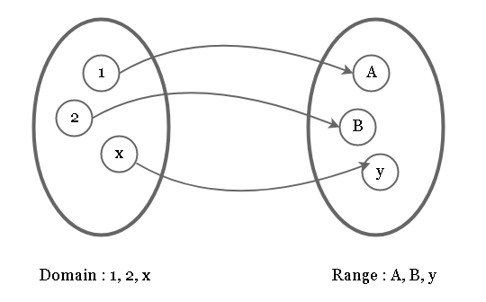
A function is a relation between two sets – set A and set B, where each element $x$ of set A is related to exactly one element $y$ of set B. Note the word “exactly” which is very important.

The elements $x$ is called domain of function (or inputs) and the elements $y$ is called the range of function( or outputs).

Rules for Function

A function must follow certain rules, otherwise it is not a function.

Every element of set A must be assigned to an element of set B.
Each element of set A must match with an element in set B.
An element of set B can be output of two or more elements of set A.
An element of set A cannot be input of two or more elements of set A. (See rule 2).

Function Diagram

What are the different ways to represent functions ?

There are 3 ways to represent functions.

Numerically – you can represent a function as set of ordered pairs (x, y) where x is the domain of the function and y is the range of the function.

For example, you can represent above diagram as

{(1, A), (2, B), (x, y)}

Algebraically – you can represent a function using algebraic notations. A function is denoted as $f(x)$ .

For example, you are given an expression $x + y = 1$ .

The above expression can be changed to following form

y = 1 - x

f (x) = 1 - x

Graphically – you can represent a function using graph. A reveal lot of information about function such a increasing function, decreasing function, odd or even and other characteristics.

To represent a function using graph find the points required to plot the graph of the function. This is done using algebraic expression of the graph.

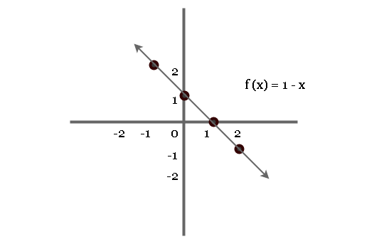
For example, let’s draw the graph of $f(x) = 1 - x$ .

x	f (x)	points (x, (f (x))
-1	2	(-1, 2)
0	1	(0, 1)
1	0	(1, 0)
2	-1	(2, -1)

The graph of the function using above points is given below.

Graph of Function f(x) = 1 – x

Piecewise-Defined Functions

A domain of a function is all real numbers. Sometimes a function is piecewise-defined. It means there are more than one function for different values of domain.

You need to specify two or more equations to represent a function with specific domain values.

For example,

f(x) = x2-1x<0x -1x\geq0

Points to Remember

If x value falls under the domain, then the function f(x) is defined for x and if x does not falls under the domain of f(x) then it is undefined for x.
When the domain of the function is not mentioned then the implied domain is set of all real numbers.
The range of the function must be a possible value after inserting x into the function f (x). The range falls between $\neg \infty$ to $+\infty$

post

Linear Equations

Linear equations form the basis for linear algebra. In the previous lesson, you learned about graph of equations plotted using points on a Cartesian plane, intercepts and symmetry of graphs.

You will learn about a graph of linear equations of two variables in this lesson.

The graph of linear equation is a straight line

\begin{aligned} &y = mx + b \\ \\ &where \\ \\ &m = slope \hspace{2px}of \hspace{2px} the \hspace{2px} line \hspace{2px} and \\ \\ &b = (0, b) = y-intercept \hspace{2px} of \hspace{2px} the \hspace{2px}line \end{aligned}

The Slope

In the linear equation, the slope is very important and tells lot about the graph. There are 4 slope condition of the line as follows

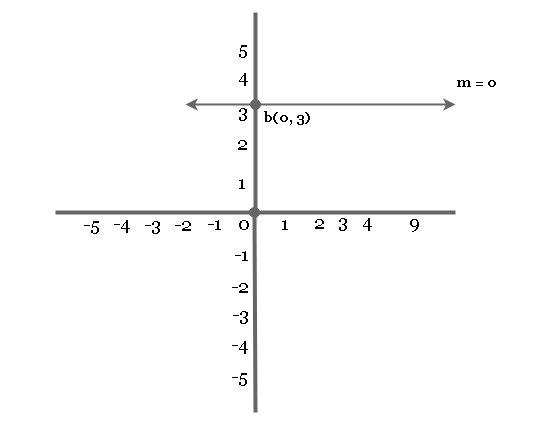
#1 Slope is Zero

Slope is $( m = 0)$ . The value of $m$ is $0$ , hence the line has no slope and it is a straight line.

Consider the equation $y = mx + 3$ , when $m = 0$ . The equation becomes $y = 3$ .

Graph of Linear Equation m = 0

Slope is greater than 0 (m > 0)

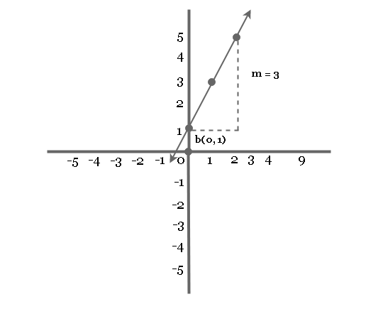
When the slope is greater than 0, then it is rising upwards. Consider the following example

y = 2x + 1

where the slope is a positive value with b = 1 as intercept value.

The graph of this equation is given below.

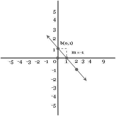
Graph of Linear Equation m greater than 0

Slope is less than 0 (m < 0)

When the value of $m < 0$ , the slope goes downwards. Consider the following example.

y = -1(x) + 1

The value of slope is $-1$ and b intercept is $(0, 1)$ .

Graph of Linear Equation m less than 0

Note: then a vertical line has no slope and its slope is undefined.

The above form of equation of a line is called point-slope form.

The Slope of a line passing through Two-Points

Suppose a line is passing through two points $(x_{1}, y_{1})$ and $(x_{2}, y_{2})$ . Then the slope of the line $m$ is given by following.

m = \frac{y_{2} - y_{1}}{x_{2} - x_{1}}

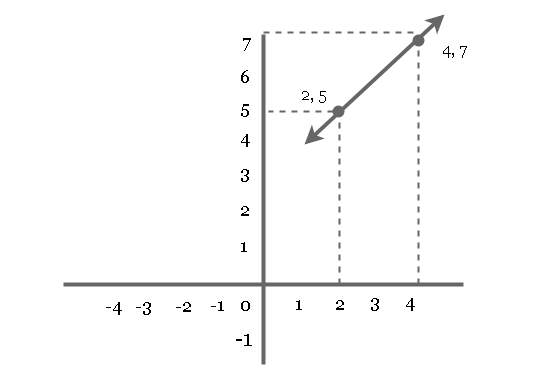
m = \frac{y_{1} - y_{2}}{x_{1} - x_{2}}

For example, Consider 2 points – (2, 5) and (4, 7). Then their slope is given by

\begin{aligned} &m = \frac{7 - 5}{4 - 2}\\\\ &m = \frac{2 }{2}\\\\ &m = 1 \end{aligned}

Therefore, the slope of the line is 1.

Slope of Line – Two Point Form

Slope of Parallel Lines ( m1 = m2)

The slope of a parallel line is same, because essentially they both are the same line just shifted above or below by few units.

Slope of Parallel Lines

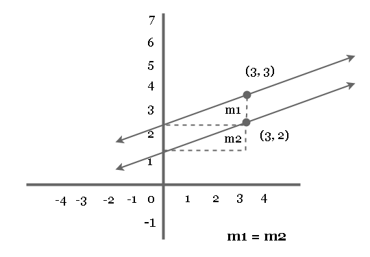
In the diagram above, both lines have the same slope. This could be proved easily using the equations of both lines.

\begin{aligned} &y_1 = m_{1}x + 2       (1)\\ &y_2 = m_{2}x + 1       (2) \end{aligned}

Consider the above example, let $x = 3$ , then the equations become

\begin{aligned} &3 = m_{1}(3) + 2  \hspace{1cm}(1)\\ &3m_1 = 1\\ &2 = m_{2}(3) + 1 \hspace{1cm} (2)\\ &3m_2 = 1 \end{aligned}

Therefore,

$m1 = m2$ for parallel lines.

Slope of Perpendicular Lines (m1 = 1/-m2)

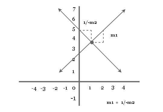
The perpendicular line make an angle of $90^\circ$ degrees. The slope of two line that are perpendicular to each other is

m_1 = \frac{1}{-m_2}

The graph of perpendicular lines shows the slopes.

Slope of Perpendicular Lines

post

Intercepts and Symmetry of Graph

In the previous lesson, you learned about graph of equations which is points on a Cartesian plane. The graph of equation has some other interesting characteristics. You will learn about two such properties in this lesson – Intercepts and Symmetry of Graph.

Intercepts

The intercepts are the points where graph touches the x-axis or y-axis. There are only two types of intercepts in a Cartesian plane.

x-intercept is given be a point $(x, 0)$ .
y-intercept is given by a point $(0, y)$ .

A graph can have no intercept, one intercept and many intercepts.

Example:

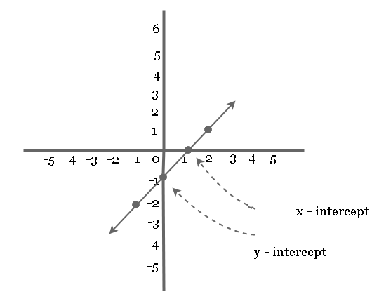
Find the intercepts of equation $y = x - 1$ and plot the graph.

Solution:

Given that $y = x - 1$ ,

You know that x-intercept the value of $y = 0$ .

\begin{aligned} &0 = x - 1\\ \\ &-x = -1\\ \\ &x = 1 \end{aligned}

Therefore,

The x-intercept of graph is point $(1, 0)$ .

Similarly,

For y-intercept the value of $x = 0$ .

\begin{aligned} &y = 0 - 1 \\ \\ &y = -1 \end{aligned}

Therefore,

The y-intercept is the point $(0, -1)$ .

Plotting the graph

To plot the graph of equation, you need to find other points on the equation.

Let’s plot the graph of equation $y = x -1$ .

Symmetry of Graph

The second property of graph is symmetry. The axis of Cartesian plane divides the graph in perfect halves is what we call as the symmetry of graph.

There are 3 rules regarding the symmetry of graph.

A graph is symmetric with respect to x-axis, whenever $(x, y)$ is on the graph $(x, -y)$ is also on the graph.
A graph is symmetric with respect to y-axis, whenever $(x, y)$ is on the graph $(-x, y)$ is also on the graph.
A graph is symmetric with respect to origin, whenever $(x, y)$ is on the graph $(-x , -y)$ is also on the graph.

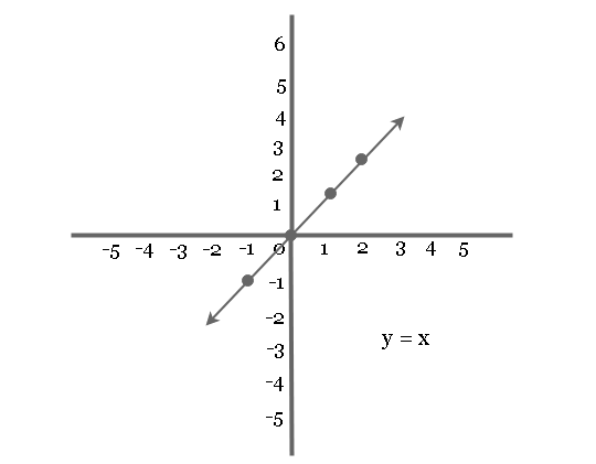
Example:

Plot graph $y = x$ symmetric to origin.

Solution:

Graph of equation $y = x$

Example:

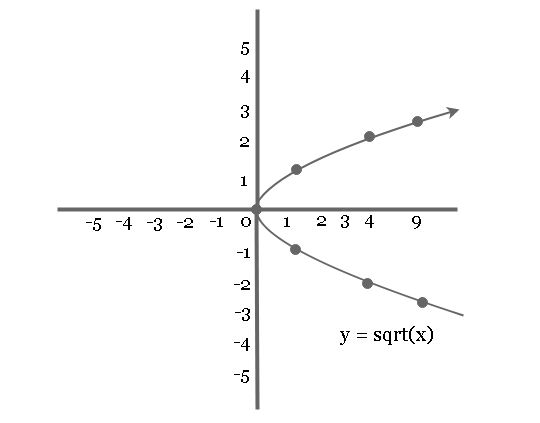
Plot graph of equation $y = \sqrt x$ which is symmetric to x-axis.

Solution:

Example:

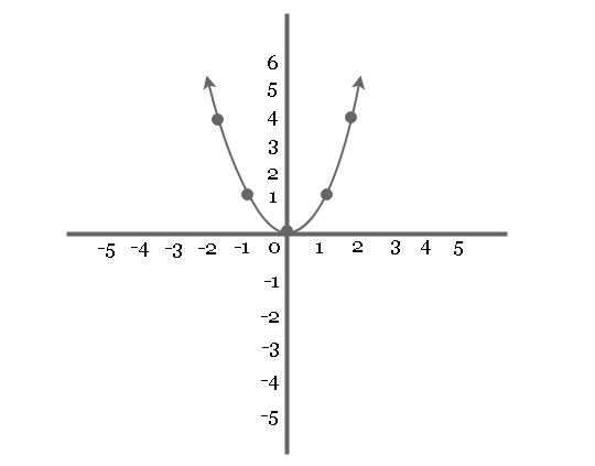
Plot graph of equation $y = x^2$ symmetric to y-axis.

Solution:

Graph of equation y = x^2

post

Graph of Equations

In the previous lesson, you learned about co-ordinate system. You know than a point is plotted on Cartesian plane with x-axis and y-axis.

A point has two values – $x$ and $y$ . For example, $p(x, y) = p(3, 7)$ is a point.

Graph of Linear Equations

Therefore, expressions involving two variable can also be plotted using the Cartesian plane known as Graph of an Equation.

So, all points that satisfy the equation will give the graph of the equation.

Example:

Plot graph of equation for $y = x + 2$ .

Solution:

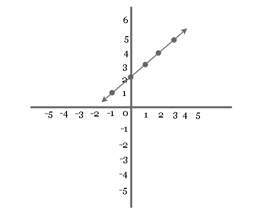
Given equation $y = x + 2$ .

You can plot the graph using co-ordinate system, but before that find all x and y values that counts as a point.

X-value	Y-value	Point
-1	1	(-1, 1)
0	2	(0, 2)
1	3	(1, 3)
2	4	(2, 4)
3	5	(3, 5)

Now, using these points you can plot the graph of the equation.

Graph of Equation y = x + 2

Non-Linear Equations

Not all equations are straight line, some equations are non-linear and give a curve for graph.Consider the following example.

Example 2:

Plot the graph of equation for $y = x^2$ .

Solution 2:

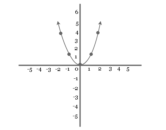
Given than $y = x^2$ .

First, you must create a table of values that represent points on the graph.

X-value	Y-value	Point
-2	4	(-2, 4)
-1	1	(-1, 1)
0	0	(0, 0)
1	1	(1, 1)
2	4	(2, 4)

You need to plot a graph using these points and each point has $x$ and $y$ values.

Graph of equation y = x^2 (Parabola)

Points to Remember:

This is something that you can try on your own.

Linear equation $y = mx + b$ has graph of line.
Quadratic equation $y = ax^2 + bx + c$ is graph of parabola.

post

x	$f(x) = \sqrt{x}$	point
4	2	(4, 2)
3	1.73	(3, 1.73)
2	1.41	(2, 1. 41)
1	1	(1, 1)
0	0	(0, 0)

$x-value$	$y-value$	$Point$
-1	-2	(-1, -2)
0	-1	(0, -1)
1	0	(1, 0)
2	1	(2, 1)