Algorithms Order Of Growth
The Big O notation, the theta notation and the omega notation are asymptotic notations to measure the order of growth of algorithms when the magnitude of inputs increases.
In the previous article – performance analysis – you learned that algorithm executes in steps and each step takes a “constant time“. You can count the number of steps and then arrive at total computing time required for the algorithm.
Background
You also learned that complexity affects the performance of the algorithm. These complexities are space complexity and time complexity.
Complexity means how do use of resources usage scale for an algorithm, whereas performance account for actual resources (e.g disk, memory, CPU time) used by algorithms during execution. Complexity affects the performance, performance does not change complexity.
If you leave fixed space like variables, constants etc, and fixed time like compile time, the complexity depends on instance characteristics (operations or steps ) of the algorithm like input size or magnitude.
What is a suitable method to analyze the algorithm?
When we consider instance characteristics which are the number of operations performed by an algorithm to solve a problem of size n.
You want to analyze three cases.
- Worst Case Performance
- Average Case Performance
- Best Case Performance
Worst Case Performance: given an instance of a problem with the maximum number of operations what is the time required for the algorithm to solve the problem. This is the worst-case analysis for the algorithm.
Average Case Performance: the instance of a problem has the average number of operations that the algorithm needs to solve. The time to complete such operations is the average case analysis of the algorithm.
Best Case Performance: the problem is already in a solved state or needs fewer steps to solve.
While analyzing an algorithm you should be more concerned about the worst case than average or best case. It is better to compare two algorithms based on the worst-case scenario.
Notations for Complexity
The number of operations for an algorithm when counted will give a function.
For example
an^2+ bn + c
This equation represents an exact step count for an algorithm. You do not need an exact count for the algorithm because when we analyze the algorithm for the worst case, consider only higher-order term and drop the lower order terms because they are insignificant when the input is huge.
therefore,
\begin{aligned}
&an^2 + bn + c\\\\
&becomes\\\\
&O(n^2)
\end{aligned}
This symbol is known as Landau symbol or $latex Big \hspace{3px} O&s=2$ notation named after German mathematician Edmund Landau. It tells us the fastest growing term in the function called the Order or rate of growth. That is why the lower order terms become insignificant and dropped.
The asymptotic notations such as $latex Big \hspace{3px} O&s=2$ is used to describe the running time of the algorithms. There are other notations to describe the running time as well.
Suppose $latex T(n)&s=2$ is the function of the algorithm for input size n,
then running time is given as
T(n) = O(n^2)
Formal Definition of Big O
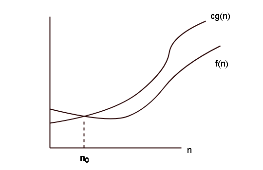
Let $latex f(n)&s=2$ and $latex g(n)&s=2$ be two functions, then $latex \mathcal{O}(g(n))&s=2$ is asymptotic upper bound to $latex f(n)&s=2$ for a problem size of n.
For a given function $latex f(n)&s=2$ , the function $latex \mathcal{O}(g(n))&s=2$is a set of functions
\begin{aligned}
&O(g(n)) = f(n) : there \hspace{1mm}exist \hspace{1mm} positive \hspace{1mm}constants \\ \\
&\hspace{1mm}c  \hspace{1mm}and  \hspace{1mm} n_0  \hspace{1mm} such \hspace{1mm}that \\\\
&0 \leq f(n) \leq cg(n),   for \hspace{1mm} all \{n \geq n_0\}\end{aligned}
The graph of the function is given by the following.
Formal Definition of Theta-Notation
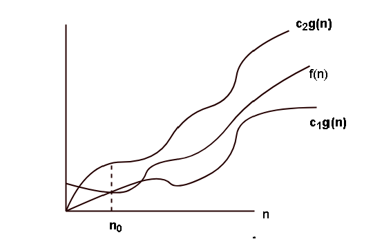
Let $latex f(n)&s=2$ and $latex g(n)&s=2$ be two functions. Then the function $latex \Theta(n)&s=2$ gives asymptotic upper bound and asymptotic lower bound, its means that the function $latex f(n)&s=2$ is “sandwiched” between $latex c_1 g(n)&s=2$ and $latex c_2 g(n)&s=2$
\begin{aligned}
&\theta (g(n)) = f(n) \hspace{1mm} such \hspace{1mm} that \\\\
&there \hspace{1mm} exist \hspace{1mm} positive\hspace{1mm} constants\hspace{1mm} c_1,c_2 \hspace{1mm} and\hspace{1mm}  n_0 \hspace{1mm} such\hspace{1mm}  that \\\\
&0 \leq c_1g(n) \leq f(n)\leq c_2g(n) for \hspace{1mm} all \{n \geq n_0\}
\end{aligned}
The graph of Theta notation is given below.
Formal Definition of Omega-Notation
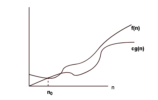
Let $latex f(n)&s=2$ and $latex g(n)&s=2$ be two functions. Then the function $latex \Omega(n)&s=2$ gives asymptotic lower bound, its means that the function $latex f(n)&s=2$ is greater than $latex cg(n)&s=2$.
\begin{aligned}
&\Omega(g(n)) = f(n) :there \hspace{1mm}exists \hspace{1mm}positive \hspace{1mm}constants \hspace{1mm}c and \hspace{1mm} n_0 \hspace{1mm}such \hspace{1mm}that \\ \\
&0 \leq c g(n) \leq f(n) \hspace{1mm}for \hspace{1mm} all \{n \geq n_0\}
\end{aligned}
The graph of Omega notation is given below.
Algorithms Complexities
Algorithm complexities and performance analysis of an algorithm is done to understand how efficient that algorithm is compared to another algorithm that solves the same computational problem. Choosing efficient algorithms means computer programmers can write better and efficient programs.
A computer resource is memory and CPU time and performance analysis revolves around these two resources. Two ways to evaluate an algorithm is listed below.
- Space requirement
- Computation time
Space Complexity
The space requirement is related to memory resource needed by the algorithm to solve a computational problem to completion. The program source code has many types of variables and their memory requirements are different. So, you can divide the space requirement into two parts.
Fixed Variables
The fixed part of the program are the instructions, simple variables, constants that does not need much memory and they do not change during execution. They are free from the characteristics of an instance of the computational problem.
Dynamic Variables
The variables depends on input size, pointers that refers to other variables dynamically, stack space for recursion are some example. This type of memory requirement changes with instance of the problem and depends on the instance characteristics. It is given by the following equation.
\begin{aligned}&S(P) = c + SP \\
&where \\
&S(P) \hspace{1mm} is \hspace{1mm}space\hspace{1mm} requirement\\
&c \hspace{1mm}is\hspace{1mm} a \hspace{1mm}constant \\
&SP\hspace{1mm} is\hspace{1mm} the \hspace{1mm}instance \hspace{1mm}characteristics
\end{aligned}
Instance characteristics means that it cannot be determined unless the instance of a problem is running which is related to dynamic memory space. The input size usually has the control over instance of a computational problem.
Time Complexity
The time complexity is the amount of time required to run the program to completion.It is given by following.
\begin{aligned}&T(P) \hspace{1mm} = compile \hspace{1mm}time\hspace{1mm} +\hspace{1mm} run-time\\
&P\hspace{1mm} is \hspace{1mm}the \hspace{1mm}program.\\
&T(P) \hspace{1mm}is \hspace{1mm}the \hspace{1mm}time\hspace{1mm} complexity \hspace{1mm}of \hspace{1mm}program.\end{aligned}
Program Execution in Steps
The computer executes a program in steps and each step has a time cost associated with it. It means that a step could be done in finite amount of time.See the table below.
| Program Step | Step Value | Description |
| Comments | zero | comments are not executed |
| Assignments | 1 step | can be done in constant time |
| Arithmetic Operations | 1 step | con be done in constant time |
| Loops | Count Steps | if loop runs n times, count step as n+1 and any assignment inside loop is counted as n step. |
| Flow Control | 1 step | only take account of part that was executed. |
You can count the number of steps an algorithm performed using this technique.
For example, consider the following example.
| Operations | S/e | Frequency | Total Steps |
| Algorithm Sum(a, n) | 0 | – | 0 |
| { | 0 | – | 0 |
| s:= 0; | 1 | 1 | 1 |
| for i:= 1 to n do | 1 | n + 1 | n + 1 |
| s:= s + a[i]; | 1 | n | n |
| return s; | 1 | 1 | 1 |
| } | 0 | – | 0 |
| Total | 2n + 3 |
Note:-
\begin{aligned}&
S/e = steps \hspace{1mm}per \hspace{1mm} execution\hspace{1mm} of\hspace{1mm} a \hspace{1mm}statement.\\
&Frequency = The\hspace{1mm} number\hspace{1mm} of\hspace{1mm} times \hspace{1mm}a \hspace{1mm}statement \hspace{1mm}is \hspace{1mm}executed.
\end{aligned}
The result of the step count is $latex 2n + 3&s=2$ which is a linear function. The performance analysis begins by counting the steps but count the steps to execute is not the goal. The goal is to find a function that will describe the algorithm in terms of its input size. This function will tell you how the algorithm will perform for different input size and magnitude.
Algorithms Pseudo Code
In this article, you will learn how to represent an algorithm using a pseudo code and elements of pseudo codes. Learning a programming language is not necessary to understand pseudo code, but knowing a programming language like C, Pascal, etc. help you understand the pseudo codes better.
Algorithms Components
The algorithm has two part – heading and the body. See the table below for more information.
| Notation | Description | |
|---|---|---|
| Heading | Algorithm <Name>(<parameter-list>) | has the name of the procedure and parameters |
| Body | { } | two braces indicates block of statements |
Example:
Algorithm Find_Max( A[n])
{

// A[n] is the list of unsorted numbers from which
// we need to  find Max value.
        max := 0;
        for i := i to n do
           if max  >= A[i] then
          {
             max := A[i];
          }
}
The above is sample algorithm to find max value from a list of numbers. The algorithm is written in pseudo code and contains lot of elements with their own notations.
Notations
See the table below to understand each notation because you need them for writing algorithms.
| Element Name | Notation | Description |
| Comments | // | start with // till the end of line. |
| Block | { } | indicate a block of statements. |
| Identifier | dummy-variable | starts with a letter, variable data type is not defined. |
| Assignments | <var> := <value> | assignments are done using := operator |
| Logical Operators | and , or , not | can use logical operators in expressions. |
| Relational Operators | >, <, <=, >=, != | relational operators are allowed |
| Single Dimensional Array | A[j] | jth element of single dimensional array |
| Multi-Dimensional Array | A[i, j] | represents a multidimensional array, (i, j) th element. |
| While loop | while <condition > do { } | a while loop structure |
| For loop | for var:= value 1 to value 2 step do { } | a for loop structure |
| Conditional statement if – then | if <condition> then <statement> | if block of statements |
| Conditional statement if – then – else | if <condition> then <statement> else <statement> | if – else block of statements |
| Input | read | command to read input values |
| Output | write | command to write output values |
| Node | node = record { data type 1 data1; data type 2 data2; node *link; } | A compound data type make of other data types |
Algorithms
Algorithms Tutorial – explore core concepts, techniques, and examples, all organized for easy learning and quick reference.
Explore Topics
Algorithms Tutorial Topics
Algorithm Basics
Learn the basic concepts of algorithms in the following section. Explore topics like pseudocode, algorithm complexity, and order of growth.”
Search Algorithms
Learn about search algorithms in following section and explore concepts like linear and non-linear search algorithms with clear diagrams and examples.
Hashing
Learn about hashing in the following section, and explore how data is mapped and retrieved efficiently using hash functions, tables, and collision-handling techniques.
Sorting Algorithm
About Algorithms Tutorial
A computer program is clear instructions in a programming language that solve some problem. You can write this program in different programming languages, but the solution to the problem irrespective of programming language remain the same. Therefore, an algorithm is an independent solution to a computer-based problem.
It is possible to automate tasks using algorithms, and creating program based on our algorithms. But, sometimes a computational problem can be solved using multiple algorithms, in which case, we have to choose the “best” or “optimized” algorithms to solve that problem.
The choice of best algorithm is based on several factors such as space to store input variables, time taken to solve the problem for a given input and so on. These are known as algorithm performance metrics. They are necessary to compare two different algorithms for best , average, and worst case scenarios.
In this tutorial you will study different types of factors that affect the choice of a good algorithm to solve a problem. You will learn about different type s of algorithm design techniques, and familiar patterns like search algorithm, sorting algorithms, etc.
Prerequisites to Learn
This guide is meant for beginner who are new to algorithms. Some experience with a programming language is sufficient to start learning algorithms, but here are some more information about prerequisites to learn algorithms.
- You must be familiar with basic mathematical concepts such as exponents, set theory, mathematical induction, trees, graphs, relations, limits and so on.
- Some knowledge of programming is recommended such as C/C++ or Java Programming.
- Knowledge of data structures is an advantage because almost all algorithms use some kind of data structures.If you don’t have the knowledge , then you should learn about stack, queues, link-lists, and trees structures at least.
You can visit our programming tutorials to learn programming concepts to get comfortable with algorithms.
[sidebar_next_prev]
Algorithm Introduction
We start with an introduction to Algorithms and its definition.
The computer program is a set of basic instructions to computer hardware. The computer hardware executes the instruction to carry out some tasks. The computer program is written using a blueprint called an algorithm. Each step in an algorithm has a clear meaning and performs a specific task.
An algorithm is any well-defined computational procedure that transforms one or more input values into one or more output values. Algorithms solve computational problems in a step-by-step manner.
For example, given a set of unsorted numbers as input, a sorting algorithm can sort the numbers in ascending or descending order as output.
\begin{aligned}
&Unsorted \hspace{1mm}set\\
&\{ 2, 3, 5, 1, 8, 4, 7, 6\} \\ \\
&Sorted \hspace{1mm}list \hspace{1mm}solved \hspace{1mm}by \hspace{1mm}sorting \hspace{1mm}algorithm\\
&\{1, 2, 3, 4, 5, 6, 7, 8 \}
\end{aligned}
Algorithm Introduction and it’s Characteristics
Algorithms have some common characteristics that separate them from computer programs. A computer program implements the algorithm to solve a computer-based problem, but the reverse is not true.
- Inputs
- Output
- Definiteness and Unambiguous
- Finiteness
- Effectiveness
Input
An algorithm needs zero or more input values to compute the outputs. The size of the input values can be different for each instance of a problem solved by the algorithm.
Certain algorithms require that you place constraints on the input values. For example, an algorithm may need only positive integers values, the negative values are not allowed.
Output
An algorithm processes the inputs and produces the desired output. The correct algorithm will always produce correct outputs for a computation problem.
Sometimes the output is a single value and sometimes it is an array of quantities.
Definiteness and Unambiguous
The algorithm must do definite operations or tasks that result in intermediate or final output. All procedures must contain unambiguous operations. If not, then the algorithm may not terminate or produce the wrong output and violate the finiteness characteristic or becomes an incorrect algorithm.
Finiteness
Finiteness means “having limits”. Every algorithm must end after a finite number of steps. It does not mean that an algorithm can take 100 steps to solve a problem because then you would not call that algorithm efficient.
An algorithm that terminates after reasonably finite steps maintains the finiteness characteristic.
Effectiveness
The algorithm must perform basic operations that can be done using a pen or pencil on a piece of paper. This is called the effectiveness of the algorithm.
How to Represent an Algorithm?
Representing algorithm depends on the context. When you are writing a new algorithm then writing steps in plain English is suitable. The best way to represent an algorithm when writing a program is using a flowchart.
Three ways to represent an algorithm are
- Language ( e.g English)
- Flowcharts
- Pseudo Code (e.g C, C++)
Algorithms in this tutorial are written in pseudo codes.The pseudo codes are inspired by programming languages like C, but they are not executable codes. Instead a mere representation of algorithm.
You will learn more about pseudo codes in future lessons.