Pthreads
Pthreads is the POSIX standard (IEEE 1003.1c) defines an API for thread creation and synchronization. It is only a specification, not implementation which a programmer can do any way they wish.
Some examples of systems using are Solaris, Linux, Mac OS X, and True64 UNIX.
Here is an example of Pthread API for constructing a multi-threaded program that calculates “summation of a non-negative integer” in a separate thread.
#include <pthread.h>
#include <stdio.h>

int sum /* this data is shared by threads */
void *runner(void *param); /* the thread that do summation */

int main(int argc, char *argv[])
{

pthread_t tid; /* the thread identifier */
pthread_attr_t attr ; /* set of thread attributes */

if (argc != 2) {
fprintf(stderr, "usage: a.out <integer value>\n");
return -1;
}
if (atoi(argv[1]) < 0) {
fprint(stderr, "%d must be >= 0\n",atoi(argv[1]));
return -1;

/* get the default attributes */

pthread_attr_init(&attr);

/* create the thread */

pthread_create(&tid,&attr, runner,argv[1]);

/* wait for the thread to exit */

pthread_join(tid,NULL);

printf("sum = %d\n",sum);
}

/* the thread will begin control in this function */

void *runner(void *param)
{
int i; upper = atoi(param);
sum = 0;

for (i = 1; i <= upper; i++)
sum+= i;

pthread_exit(0);
}
The main program has a Pthread header included. The variables Pthread_t and pthread_attr_t are thread identifier and attributes for the thread.
The pthread_attr_init(&attr) sets the default attributes for the thread.
pthread_create(&tid, &attr,runner, argv[1]);The above will create a new thread which is the runner function. The main function is the main thread that creates the second thread runner. Both threads run in its own function. Once control return to the main thread, it prints the results and exit thread – pthread_exit();.
References
- Abraham Silberschatz, Peter B. Galvin, Greg Gagne (July 29, 2008) Operating System Concepts, 8 edn., : Wiley.
- Tanenbaum, Andrew S. (March 3, 2001) Modern Operating Systems, 2nd edn., : Prentice Hall.
Multi-threaded Programming
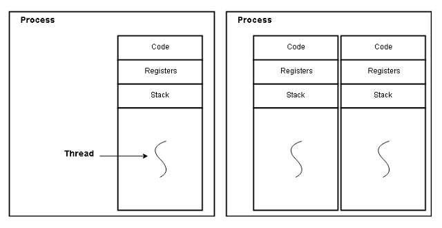
A thread is a basic unit of CPU utilization; it has a thread id, a program counter, a register set, and a stack. It shares code, data and other os resources such as open files and signals with other threads in the process.
Multi-threaded Processes
The traditional single-threaded program can do only one task, the multi-threaded process can do more than one tasks at a time.
For example, if a web server handles multiple users, rather than creating multiple similar processes, it could create multiple threads for multiple users. Many OS is multi-threaded and each thread performs a specific task at the kernel level.
Advantages of Using Multi-threaded Programming
There are many advantages of using multi-threaded programming which are:
- Responsiveness – One part of a process is blocked, while other threads interact with users doing another task.
- Resource sharing – Threads share codes, data and memory to each other by default.
- Economy – It is easier to create and manage thread than process because the threads use same address space as the process, sharing data is easier for threads, than inter-process communication.
- Scalability – You can run different threads on different processors in multi-processor systems.
Multi-Threading Models
Since the processes are different and run in different modes their threads also run in respective modes. The kernel thread supports the user-thread. The multi-threaded model defines the relationship between user-thread and the kernel-thread.
1. Many-to-One Model
2. One-to-one
3. Many-to-many
Many-To-One Model
Many user threads map to one kernel-thread in this scheme. A thread library at user space manages the user threads. A blocking system call from one thread will block the whole process.
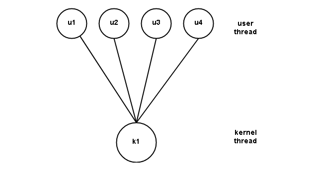
Only one thread can access the kernel thread at a time, hence, parallel execution of threads not possible in multiprocessors system.
One-To-One Model
This model maps each user thread to a kernel thread. Unlike the many-to-one model, it allows parallel execution of user threads on multiprocessors.
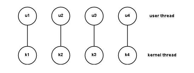
There is a performance overhead when a new thread is created because we also required to create a kernel thread. So to implement this model, the OS must restrict the number of threads. Linux, as well as Windows OS, implement this model.
Many-To-Many Model
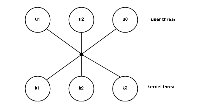
Maps many user threads to a smaller or equal number of kernel threads. This model is better than other models and achieves true concurrency.
Two-Level Model
The two-level model is a variation of many-to-many model used in some operating systems such as HP-UX, True64 UNIX, IRIX, and older versions of Solaris (prior to Solaris 9).
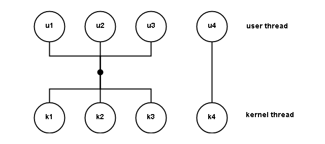
The user threads are supported by smaller or an equal number of kernel threads, and also allows one-to-one mapping with kernel thread.
Thread Libraries
Thread library provides API to create and manage threads. The library is implemented at the user level space or the kernel level space depending on the OS.
API - application programming interface is a set of functions to build applications.Two ways to implement a thread library.
1. Library at userspace with no OS support.
2. Kernel level with OS support.
There are three thread libraries in use today. Here is the list:
1. POSIX Pthread
2. Win32
3. Java
In the next article, we will discuss the above three libraries in detail.
References
- Abraham Silberschatz, Peter B. Galvin, Greg Gagne (July 29, 2008) Operating System Concepts, 8 edn., : Wiley.
- Tanenbaum, Andrew S. (March 3, 2001) Modern Operating Systems, 2nd edn., : Prentice Hall.
Operating System Structure
OS provides the computing environment. They are organized in many ways in different systems, but a few things are common for all OS.
In a single user system, the CPU sits idle when I/O is working or vice-versa. The CPU utilization increase with multi programming systems. A subset of jobs from a pool of jobs on the disk is loaded into the memory. The CPU executes one of them if the job has to wait for CPU switch to another job and later come back to the first job when the wait is over.
Different Systems
The multiprogramming system does not allow user interaction with the system. A time-sharing system allows multiple users to interact with the system directly. The time-shared computer switches between programs from different users so frequently that it gives an impression to the user that the entire system of dedicated to him.
The multiprogramming and time-sharing system must make decisions about two things:
1. several jobs ready to be brought to memory from the pool. (job scheduling)
2. several processes ready to run at the same time. (CPU scheduling).
The time-sharing system gives good response time by swapping process in or out of disk. Another method is a virtual memory scheme which abstracts physical memory into much larger logical memory. thus allowing programs larger than physical memory to run without problem.
Time-sharing system must provide a file system on the disk. It must also ensure that operations are synchronized and processes are cooperating. The system must prevent a deadlock situation.
Operating System Operations
Modern OS is interrupt driven. OS waits for events that are created by an interrupt or a trap. A trap or an exception (divide by 0) is a software interrupt caused by an error or user program request for specific OS services. An interrupt service routine from OS handles the interrupt.
OS and user programs share common resources, any erroneous program can change other programs, or data of other programs, or even OS itself. Therefore, some kind of protection is necessary to protect OS codes.
Dual-Mode Approach
To protect OS codes, we must be able to distinguish the OS-specific codes and user-defined codes. The computer hardware can differentiate the codes. It is divided into two modes of execution – user mode and kernel mode. The kernel mode is also known as supervisor mode, system mode, or privilege mode. A mode bit is added to computer hardware to indicate the current mode – kernel(0) and user(1).
When the user is executing an application, it is in the user mode and when the application requests an OS service (system call) it is in kernel mode.
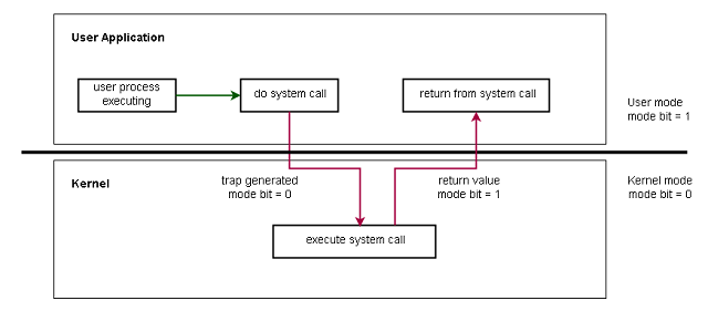
The system boots in kernel mode and runs an application in user mode. When a trap or an interrupt happens the mode bit is set to 0 before transferring the control to OS for system calls. The mode bit is set to 1 when OS returns to the user program. The hardware ensures that faulty program does not run instructions in privileged mode, and only privileged instructions must run in kernel mode, otherwise, consider that illegal and generates a trap.
Except for MS-DOS, all modern operating systems such as Windows XP, Windows Vista, Windows 7,8,10, Unix, Linux supports dual-mode of protection.
Operating-System Services
An operating system manages the computer system resources for smooth and efficient execution of user applications. An OS provides services such as
- Process management
- Memory management
- Storage management
- Caching
- I/O system
Process Management
A process is a program in execution that needs CPU time, memory, and i/o systems. The user process is different from the system process because the system process belongs to OS. The process management activities of OS are:
- Process and thread scheduling for CPU.
- Creating and deleting processes.
- Changing process states – Suspending and resuming.
- Process synchronization for concurrency.
- Process communication – interprocess communication.
Memory Management
The memory management task deals with managing the main memory which is a large array of words with each word having its own address. During the instruction-fetch cycle, the CPU read instructions from the main memory, and during the data-fetch cycle, it read data from the memory. If the data is on the disk then it must be brought to the main memory because CPU has direct access to main memory.
A program is also loaded from disk to main memory so that the CPU can read the instructions and data as mentioned earlier. Once the program terminates, the memory is free and available to other programs. Since several programs run in memory, there is a need for memory management scheme which many factors such as system design, hardware support, etc.
The memory management activities are:
- Track which memory location is used and by whom.
- Decide which process and data to move in or out of memory.
- Allocate or Free (deallocate) memory as required.
Storage Management
The storage management is about preserving information that is not in main memory. The storage device keeps information in the form of bits or bytes. However, the OS gives a logical view of this information in the form of files. There are many types of files depending on what information gets stored there – text, image, or video. So the main task of OS is file management.
The file management activities are :
- Create or Delete files
- Create or Delete directories for file organization.
- Support all primitives storage technologies for file or directory manipulation.
- Mapping files onto secondary storage(disk).
- Backing files on a stable storage device.
- Free-space mangement
- Storage allocation.
- Disk scheduling.
Caching
The caching is faster memory and the first place where CPU looks for information. It is because the main memory is slower most of the time, so if need any information quickly it is kept in cache for quick access. This avoids the need to access the main memory again for the same information.
Cache management is a design problem, we must select the right cache system – software cache or a hardware-based cache and replacement policy that decides which information to be stored in the cache. The size and replacement policy of the cache can also increase the performance of a system.
I/O Systems
The role of OS is to hide details of hardware devices from the user. In Unix, the details of devices are hidden from OS itself by the I/O subsystem. The I/O subsystem consists of :
- A memory management component that does spool, buffering and caching.
- A device driver interface.
- Drivers for specific devices.
All device-related tasks are controlled by device drivers, and only it knows the peculiarities of the device.
Protection and Security
Access to data must be regulated due to multiple users and concurrent execution of processes.
For example,
- Memory addressing hardware ensures the process runs in its own address space.
- The timer ensures that the process must relinquish its control after some time.
- Device control registers are inaccessible to users thus protecting the peripheral devices.
Protection is controlling access to resources by processes and users. OS must specify the controls and give means to implement these controls. Protection-oriented systems can distinguish between authorized and unauthorized users but still fails due to inappropriate access.
Security incidents are common in computing environments. In such cases, the OS must defend the system with proper security. The modern OS maintain a list of UID (user identification) numbers or user IDs with a password to secure the system. Sometimes, the user identification is made of SID (security ID).
The modern file system allows users to set access rights for the files they create or own. They can give read, write, and modify or any combination of these three.
References
- Abraham Silberschatz, Peter B. Galvin, Greg Gagne (July 29, 2008) Operating SystemConcepts, 8 edition edn., Wiley.
- Tanenbaum, Andrew S. (March 3, 2001) Modern Operating Systems, 2nd edn., Prentice Hall.
Computer System Structure
The computer system structure consists of interrupt mechanism for I/O devices, memory unit to run programs, memory protection, and disk storage to save program and data files.
Computer-system operations
A modern general purpose computer has CPU and device controllers for devices such as disk, audio devices, and video display devices connected to a common system bus. Each controller is for a specific device only and it has a local buffer.
The CPU and device controllers can run concurrently and compete for memory. A memory controller synchronizes access to shared memory.
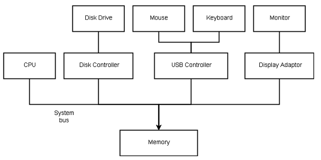
When a computer starts it initiates a simple program called the bootstrap program stored in a read-only memory (ROM) or erasable programmable read-only memory (EPROM). The bootstrap is a simple program that initiates the system and loads the OS in memory. The OS waits for an event called.Interrupt
There are two types of interrupts – hardware and software interrupt. The hardware generates interrupt by signaling the CPU directly. A software interrupt is performed by a system call also known as monitor call. The CPU stops current operation and transfer the control to a fixed memory location where interrupt service routine (ISR) for the interrupt is located. Once interrupt service routine finished execution, the CPU resume the control of the interrupted operation.
Two things are very important, no matter how OS is designed:
- CPU must efficiently transfer the control to ISR.
- Speed up the process of transfer.
The ISR can call an interrupt handler to check the appropriate handler, but it is not necessary because there are few fixed addresses for ISRs. Hence, a table of pointers to the ISR address called isInterrupt vector maintained. The indexed interrupt vector immediately transfers the control to the correct ISR of a device upon receiving interrupt request.
The interrupt mechanism must save the address of the interrupted instruction in a fixed memory location, or a stack and load this address to program counter once the interrupt routine is completed. This will appear as if the interrupt never happened.
Computer Storage Structure
The computer storage consists of two main memory – primary memory or main memory and secondary memory/disk drives. The program is loaded into a rewritable main memory called RAM (random access memory). The memory is organized using words where each word has its own memory address
A computer based on Von Neumann architecture reads an instruction in CPU registers and decode the instruction and fetch the required operands from memory and store the result back to the main memory. The main memory and registers are primary storage because the CPU can access them directly if they are not accessible, then it must be brought to the memory before the CPU can manipulate them.
There are two concerns while CPU access the memory addresses:
- Speed of memory access
- Memory access protection
The CPU is very quick in fetching and decoding the instructions, but of the operands are not in registers, the memory fetch could delay the CPU operations. Cache memory is faster memory that can speed up the memory access.
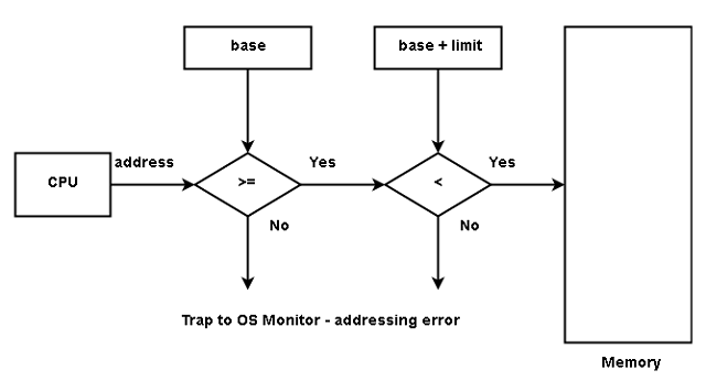
Secondly, each program must use its own memory space, otherwise, it would be illegal access and result in a program crash. To protect memory we use two registers – base register and limit register.
The base register contains the starting memory address of a process and limits register contains the size of the range of addresses for the process. See the figure below.
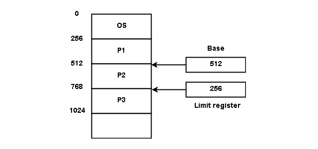
For example, base register = 512 and limit register = 256
Then the process P2 in the above figure can only access all addresses from 512 to (512 + 256) = 768. If the program tries to access any other address outside this range, an interrupt happens.
Therefore,
\begin{aligned}
Legal \hspace{1ex}address >= Base \hspace{1ex}register \hspace{1ex}value\\ \hspace{1ex}AND < (Base\hspace{1ex} register\hspace{1ex} value + Limit \hspace{1ex}register \hspace{1ex}value)\end{aligned}
Any address generated by user application is verified by CPU hardware with the registers if the user application tries to access operating system memory address the OS trap is generated. The OS loads the base register and limit register and has the ability to modify the address because OS runs in kernel mode. The application which runs in user mode cannot access the registers. You will learn about user mode and kernel mode in the next article.
Logical address and Physical address
A logical address is also called a virtual address because it is user generated. The virtual address is mapped to a physical address which is the real memory address with the help of base and limit registers.
For example, suppose
\begin{aligned}
&Base = 3000\\
&Limit = 1500\\
&Legal address >= 3000 < 4500
\end{aligned}
If the virtual address is  , then the OS generates a physical address of
  . This address is within the limit of
  .
.
The memory space is very less and only include programs that are running. What about the programs that are not executing currently? Where do we store them? Such programs are in the form of files and stored in secondary storage devices called tape or disk drives.
Disk Storage Structure
Magnetic tape or disk is called a secondary storage device. It has huge space compared to the main memory space. The disk storage device comes in various sizes, sometimes more than 1 terra bytes disk is used in computer systems.
Though the magnetic disks have large space when compared to main memory, the magnetic disks are slower to access. It takes more CPU time to perform an I/O operation than a CPU bound memory operation.
For this reason, the CPU remains idle most of the time in a single user system. In a multi-tasking system, the CPU can process another user. In the next article, you will learn about OS structure and how CPU performance is optimized in a time-sharing computer.
References
- Abraham Silberschatz, Peter B. Galvin, Greg Gagne (July 29, 2008) Operating SystemConcepts, 8 edition edn., : Wiley.
- Tanenbaum, Andrew S. (March 3, 2001) Modern Operating Systems, 2nd edn., Prentice Hall.
OS System Calls
A system call is an interface between the user program and the operating system. The program asks for different services and in response the OS invoke a set of system calls to fulfill the request.
What is a system call?
A system call is written in either assembly language or a high level such as C, Pascal and so on. If high-level language is used, then system calls are predefined functions or subroutines that can be invoked directly by the OS.
For example,
A user wants to copy information from an input file to an output file. There are three stages to this task listed below:
- Input-Output file names
- Open the files and perform read-write
- Close all files
Each of the above stages requires the OS to provide necessary services. The OS request for the input file name which will invoke a set of system calls and if the file already exists, then continue to the next stage. Suppose output file exists then OS will delete it and create a new file.
To open the file an open() system call is invoked, followed by reading () and write() call to perform the read-write operation. You may need to supply the parameters for a system call, rather than calling it directly in some OS.
Once the task is completed, the files are closed using close() system call.
In case of errors, interrupts, or unexpected termination of a system call, another set of system call respond to the errors by reporting it to the user on the computer screen.
Passing parameter to system calls
There are three ways to pass parameters to OS (system calls):
- The parameter passed to registers
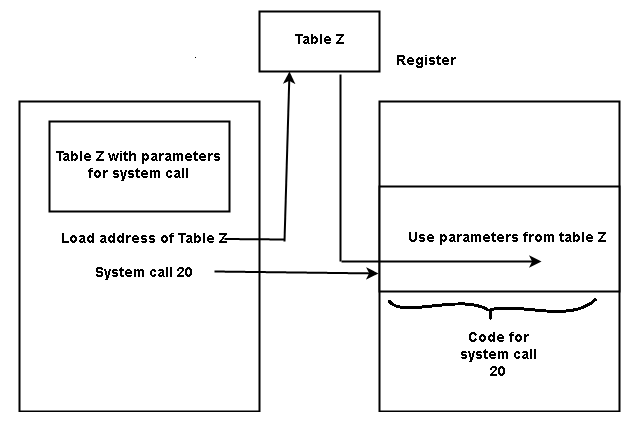
- Parameters stored in block or table in memory and the address of the block is passed to OS.
- The parameter is pushed on or off the stack by OS
Types Of System Calls
The system calls are divided into the following types:
- Process and job control
- File manipulation
- Device manipulation
- Information maintenance
- Communication
Process and Job Control System Calls
These types of system calls are related to process and job. The process either terminates normally (end) or abnormally(abort). If the process terminates abnormally that causes an error trap, a memory dump is generated an error is reported. The memory dump available on disk can be used for debugging. The process terminates and transfers control to the command interpreter which continue the execution of the next command. In a batch system, the command interpreter skips the job and continue with the next job. In a GUI based system, popup reports and asks for further action.
A process can load (load()) and execute (execute()) another program or process. The control is returned to the old process when the new process terminates. We save the memory image of the old program files so that next time it calls the new program again when executed.
If both old and new program runs concurrently, it means that a new process is created. You can create a process(create() or submit job) explicitly. When we create process, we should be able to control attributes of the process such as getting attributes(get process attribute) or reset (set process attribute) the attributes of the process.
A process must wait(wait time) for sometimes for other processes to finish or it must wait for some event (wait event) to happen before continue with the execution. A process must signal other process of events by signal (signal event).
Two process running concurrently share data and to avoid conflict one of the process lock the shared data to avoid inconsistencies in updates. This is done using aquire lock and release lock command.
Examples:
We give two examples for process control calls – MS-DOS System and FreeBSD UNIX.
MS-DOS is single user system that runs program directly and does not create new processes. The program runs and terminates successfully, or an error trap happens which is saved to memory. The command interpreter reloads and display error to the user.
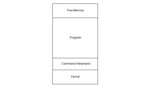
FreeBSD system is time-sharing or multi-tasking system. Each user who logs into the system gets a shell which is similar to MS-DOS command interpreter. The command interpreter request user input and runs the program. A new process is created using fork() system call and the selected program is run using exec() call. Either the process completes, or it runs in background, while the shell waits for next command. The user can run another program.
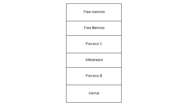
The process terminates using exit() system call which return a 0 to parent process.
File Management System calls
there are several system calls that deals with files. We should be able to create and delete files. The system call may require file name and sometimes few attributes. The must be opened to perform read, write, or reposition (rewinding or skipping the end of file). After the job is done the file must be closed.
The operating system provides system calls to manipulate file or directory attributes. The most important system calls are getting file attribute and set file attribute.
Some OS provides APIs to move and copy files using system calls. There are system programs using code and API to do those tasks.
Device Management System Calls
A process requires resources such as memory, disk, files access, etc. If resources are available the system process continues to return the control to the user process. Otherwise, the process waits for the resources until its available.
Each resource can be thought of as a physical device(disk) or virtual device (files). In a multitasking system, the user needs to request a resource to exclusively use it and release it after use.
Once device access is granted, we can read, write, or reposition the device. I/O devices and files are almost identical to OS and combined into device structure file, hence there are a common set of system calls for both as in case of UNIX. Otherwise, device files are kept in separate directories, given special names, or attributes to identify them.
Information Maintenance System Calls
These types of system call transfer information between the user program and the operating system. For example, the system call returns current date and time, OS version number, free disk space, free memory, etc.
When a program crashes a set of system call creates a memory dump useful in debugging the program. An operating system provides a time profile of a program that indicates the time spent at a location or location set. When a timer interrupt happens the value of the program counter is recorded which gives the time statistics of the program.
Communication System Calls
The process must communicate with each other for co-operation. There is two such model – Message passing and Shared memory. The system calls of this type help in interprocess communication. Inter-process communication is a topic for another article.
References
- Abraham Silberschatz, Peter B. Galvin, Greg Gagne (July 29, 2008) Operating SystemConcepts, 8 edn., Wiley.
- Tanenbaum, Andrew S. (March 3, 2001) Modern Operating Systems, 2nd edn., : Prentice Hall.
- Sweta Verma (2009) Krishna’s Operating System, Meerut: Krishna Prakashan Media (P) Ltd.
Process Concepts
A process is program in execution in a modern time-sharing computer. A process needs resources such as CPU, memory, and input-output devices. OS is responsible for creating, deleting, and maintaining process information.
Understanding Processes
Therefore, we can safely say the following things about the process:
- A process is an instance of a program in execution in a time-sharing computer.
- All processes are executed sequentially.
- A process may or may not call another process.
- A process is an ongoing activity of computer, defined by the program counter and data contents of processor registers.
Each process gets address space (virtual) which consists following:
- Stack address space
- Data address space
- Space for source code
See the figure below.
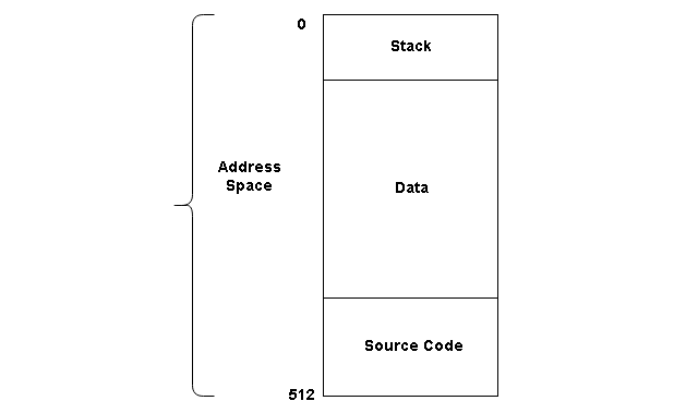
Stack Address space – The stack space is used for functions and system calls. The system calls are functions that belong to OS.
Data Address Space – A process will not execute unless all the required information is available. The process keeps both static and dynamic allocated variables in its data space.
Source Code Space – The source code section contains read-only code so that the process does not modify it. This address space contains only text information.
Many instances of a program mean multiple addresses will be created, one for each instance.
Process Operations
The operation on the process is:
- creating a new process
- terminating a process
Every time a new process is created it gets an ID. The getpid() and getppid() allows a process to get their process id. A process is created by OS as soon as a program is loaded into the memory. The OS provides the necessary resources for the process. The running process can change state and can be terminated using various system calls.
fork()
Creates a new child process which is a copy of the parent with a new pid. The child process gets its own pid, address space, but return different values.
exec()
The exec() runs a list of system calls and replaces the current process with a named program. The entire address space of the current process is replaced with a new program.
signal(), kill(), exit() and abort()
The,signal()kill(), exit() and abort() terminates the process and claim the resources of the terminated process.
Process Control Block (PCB)
The OS represents a process with a process control block, also known as the task control block. It contains the following information about the process.
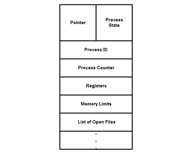
Process state – A process could be in any state after it is created such as new, ready,
Process ID – Every new process gets a unique number called process ID to uniquely identify the process.
Program Counter – It contains the address of the next instruction to be executed.
CPU Registers – When an interrupt occurs the current process state is saved, this allows the process to continue later.
CPU Scheduling information – The PCB contains process scheduling information in the form of process priority, a pointer to scheduling queue, and other process scheduling information.
Memory Management Information – Depending on the memory management technique, PCB contains information such as the address of base and limit registers, segments tables or page tables.
Accounting Information – This information includes CPU usage, account number, process number, and so on.
I/O Status – It includes a list of devices assigned to the process and list of open files, etc.
References
- Abraham Silberschatz, Peter B. Galvin, Greg Gagne (July 29, 2008) Operating System Concepts, 8 edn., : Wiley.
- Tanenbaum, Andrew S. (March 3, 2001) Modern Operating Systems, 2nd edn., : Prentice Hall.
Operating System Concepts
An operating system is system software that ensures the smooth functioning of a computer system.
In earlier days of computing, the only job of a computer was to compile source code into a program. There were programs to do other tasks such as printing, loading source code, etc. These programs are called system programs because they interact with hardware on behalf of users.
How Operating Systems Evolved
The first generation computers run programs that were written in machine language.
The batch system allows running similar programs into batches where control is automatically transferred to the next job in the batch. A user cannot interact with the system directly or the job.
The CPU utilization is still low in a batch system because jobs that are Input/Output bound have to wait for the device to complete and CPU remains idle during this time. Therefore, the batch system is suitable for a batch queue with bigger jobs.
The multiprogramming system is based on the fact that if CPU or I/O (input-output devices) is waiting, then it must switch to a job from other users increasing the overall utilization.
The time-sharing system is a kind of multiprogramming system where all users interact with the system at the same time. This is because the switching between jobs is so fast and efficiently time-based.
The system programs are bundled into a system software called an operating system. We have listed below the primary activities of an OS.
- The operating system is also a resource manager. It allocates an appropriate amount of CPU time, memory, disk space to each program.
- An OS must ensure that each program should run in its own space without crashing other programs. The hardware system must support such functionality.
- Ensure high performance through scheduling programs and its activities.
Parts of a Computer System
A computer system has four important components or parts. Each of these components interacts with each other to get a computational job done.
- Users
- Application programs
- Operating systems
- Hardware systems
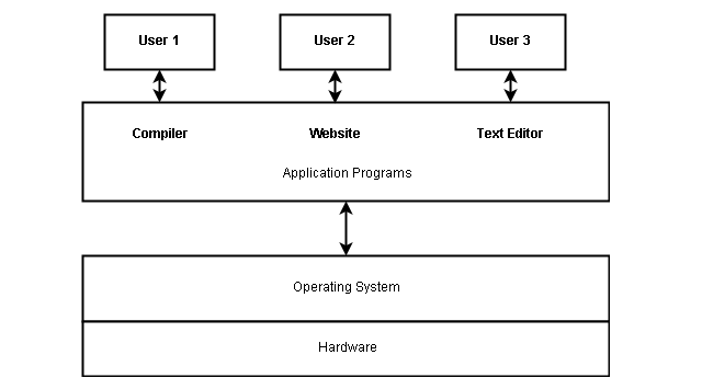
Users – The users run the application programs and provide the input data. Users receive the output of the application.
Application programs – They solve a specific computing problem for the users, by utilizing hardware resources of a computer.
Operating System – It manages the resources for application programs and control user inputs.
Kernal – It is the core of an operating system that always runs in the main memory. It has all the frequently used functions.
Hardware – The processor, the disk, the memory, and the input/output devices are the resources for solving computing problems.
Services provided by OS
An operating system resource manager provides many services listed below.
- Process creation
- Execute programs
- Control user input/output
- File access control
- System protection and security
- Accounting
All of these are discussed in more detail in future articles.
References
- Abraham Silberschatz, Peter B. Galvin, Greg Gagne (July 29, 2008) Operating SystemConcepts, 8 edition edn., Wiley.
- Tanenbaum, Andrew S. (March 3, 2001) Modern Operating Systems, 2nd edn., Prentice Hall.
Disk Scheduling Algorithms
In this article you will learn about storage structure and disk scheduling algorithms. You analyses the advantages and disadvantages of different disk scheduling algorithms. Learn to measure the performance of disk such as seek time.
A problem is given for each algorithm, you can also try to solve them if you are already familiar with the concepts.
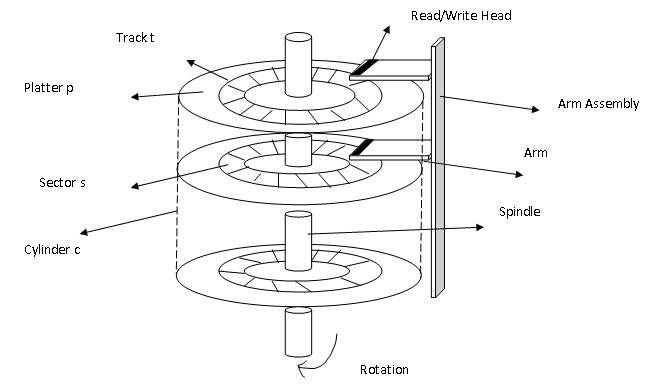
A surface of the circular platter is divided into tracks and tracks are subdivided into sectors. A storage capacity of the disk is measured in GB. The disk rotates 60 to 200 times per second. The transfer rate is the rate at which data transfer between disk and computer.
Positioning time or random-access time is the time necessary to position the arm to the desired cylinder called the seek time.Time taken for the sector to rotate to the disk head is rotational latencies. Both seek time and rotational latencies are of several milliseconds.
The distance between the disk head and the platter is very less (microns) and the head sometimes comes in contact with the disk surface damaging it. This accident is called the head crash.
Removable disks
They work like the normal Hard disks and their capacity is measured in GBs. Some disks are attached to the computer using Buses and their type as follows.
- EIDE – Enhanced Integrated Drive Electronics
- ATA – Advanced Technology Attachments
- SATA – Serial ATA
- USB – Universal Serial Bus
- FC – Fiber Channel
- SCSI – Small Computer-System Interface
Data transfer is carried out by a processor called the controller.
Host controller – computer end of the bus
Device Controller – built into the each disk drive.
Disk Structure
Modern disk drives are accessed as a logical block which is the smallest unit of transfer. A block may be of 512 bytes, but some disks are low-level formatted and have 1024 bytes block size.
One dimensional array of a logical block is mapped to sectors, starting from sector 0 which is the first sector in the first track of outermost cylinder. The mapping proceeds to other cylinders in this way from cylinder 0 to N-1.
What is the use of such mapping?
Using the block address we can find the cylinder and track number and sector number on the track. Such a translation is difficult because some disk may have defects and second, number of sectors per track is not a constant.
A track in an outer zone has more sectors than inner tracks. It has 40 % more sectors. To read and write at a constant speed, either keep the head constant and increase or decrease the rotation speed of the disk.
Otherwise, keep the rotational speed same and change the density of bits as the head moves from inner track to outer most track ( constant angular velocity).
Disk Attachment
- Host –Attached Storage
- Network-Attached Storage
Host Attached Storage
It is accessed through local I/O ports of a computer. Desktop PC uses I/O bus architecture called IDE or ATA, SATA etc.The high-end server uses SCSI or FC (Fiber channel). SCSI is a bus architecture and SCSI protocol supports 16 devices per bus.
SCSI Initiator – The host which has a controller card.
SCSI target – SCSI disk drives are the targets.
Physically it is a ribbon cable with a large number of conductors. FC is high-speed serial architecture and uses fiber cable or a 4 -conductor copper cable. It is mostly used in SAN storage.
Network Attached Storage (NAS)
It is a special purpose storage system that is accessed remotely over a data network. Clients access NAS using RPC interface and RPC is carried via TCP or UDP over IP network such as a LAN. iSCSI is another NAS that carry SCSI protocol over an IP network.
Storage-Area-Network (SAN)
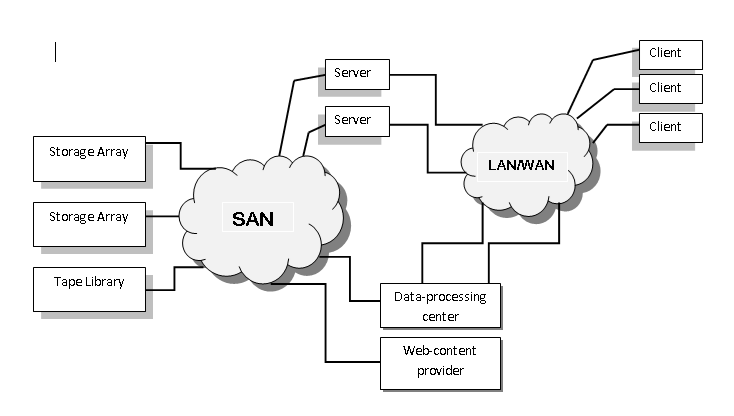
SAN is a private network using storage protocols rather than networking protocols. It connects servers and storage together. Multiple hosts and Storage arrays can connect to same SAN and it can be dynamically allocated to hosts. SAN has more ports and less expensive ports than the storage array ports and SAN switch control the access to storage by hosts.
Disk Scheduling
The disk access time has two components – seek time and rotational latency.
Disk Bandwidth – It is the total number of bytes transferred divided by the total time between the first request for service and last transfer.
By scheduling the disk access we can reduce the time a process has to wait for disk operation to complete. In multi-programming, the number of a process request for disk device access and if the device is already processing a request the process has to wait in the device queue with other pending requests.
FIRST COME, FIRST SERVE
It is not an efficient algorithm but it is fair in scheduling the disk access. For example, we are given a list of request for disk I/O to blocks on a cylinder.
98, 183, 37, 122, 14, 124, 65, 67If the starting point is 53 then the access would be like below
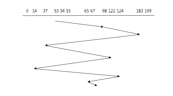
The big jump from 183 to 37 could be avoided if somehow 14, 37 and 122, 124 are served together. This indicates the problem with the FCFS algorithm which is larger head movement.
SSTF SCHEDULING
The main idea of the Shortest-Seek-Time-First algorithm is to service all the requests close to the current position of the head before moving far away to service other requests.
Example:
Considering our previous sequence of disk blocks access.
Queue = 98, 183, 37, 122, 14, 124, 65, 67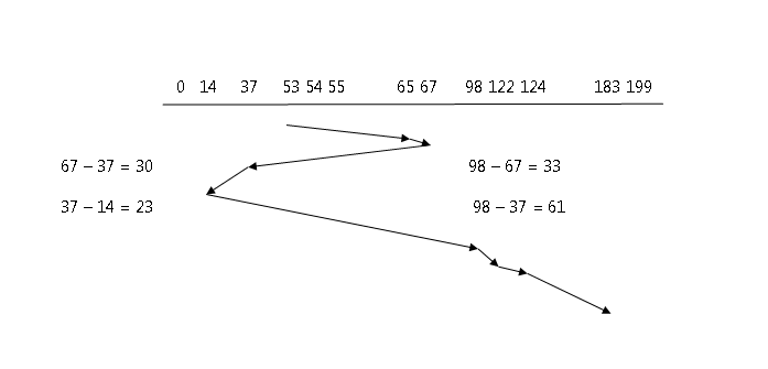
There is a substantial improvement compared to FCFS algorithm. The total head movement is as follows.
65 – 53 = 12 37 – 14 = 23 124 – 122 = 2
67 – 65 = 2 98 – 14 = 84 183 – 124 = 59
67 – 37 = 30 122 – 98 = 24
Total Head Movement = 236 cylinders.
But suppose 14 and 183 are a queue and a request near 14 came, it will be served and next one is also close to 14 came, it will be served first and this will lead to starvation of 183 in the queue. SSTF is an improvement but not the optimal algorithm.
SCAN SCHEDULING
In this algorithm, the disk arm works like an elevator starting at one end servicing all the way up to the other end and then start from the other end in reverse order.To use the SCAN algorithm, we need to know two information.
- Direction of Scan
- Starting point
Let’s consider our example and suppose the disk start at 53 and move in the direction of 0.
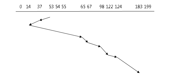
Total Head Movement
53 – 37 = 16 67 – 65 = 2 124 – 122 = 2
37 – 14 = 23 98 – 67 = 31 183 – 124 = 59
65 – 14 = 51 122 – 98 = 24
Total head movement = 158
The SCAN move in one direction and service all the request immediately, but while returning in reverse direction it does not serve any request since they have been serviced recently. More of the request is at the opposite end, we will see an algorithm that wants to go the other end directly.
C-SCAN ALGORITHM
In this algorithm, the head from one end to the other servicing request along the way, however, it does not do a reverse trip and go to the beginning directly as if it is a circular queue.
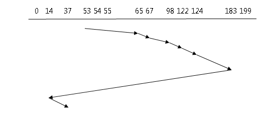
Total Head Movement
183 -124 = 59 98 – 67 = 31 183 – 14 = Look for Request
124 – 122 = 2 67 – 65 = 2 37 – 14 = 23
122 – 98 = 24 65 – 53 = 12
Total Head Movement = 153
LOOK SCHEDULING AND C-LOOK SCHEDULING
SCAN and C-SCAN not implemented as they described earlier, but they move to one direction and reverse its direction of movement rather than directly going to the beginning.
References
- Abraham Silberschatz, Peter B. Galvin, Greg Gagne, A Silberschatz. 2012. Operating System Concepts, 9th Edition. Wiley.
- Technology, Illinois Institute of Technology. n.d. Disk Scheduling Algorithms. Accessed 7 24th, 2016. cs.iit.edu.
Deadlock Prevention With Banker’s Algorithm
In this article, you will learn about deadlock prevention method – Banker’s algorithm and Resource allocation graph. You will also learn about 4 conditions for deadlock.
Let’s start with the resource allocation graph.
Resource Allocation Graph
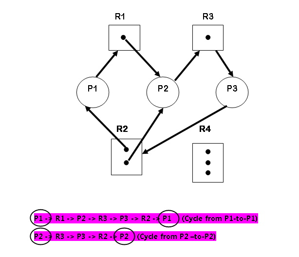
Resource Allocation graph describes the deadlock more precisely. It has a set of vertices V and set of edges E.
Vertices types
Vertices are divided into
 set of active processes in the system.
 set of vertices that represent the resources.
Edge types
 means
means  has requested resource
  and waiting for it is called request edge
 means that the instance of resource is allocated to process called the assignment edge.
Resource  may have more than one instance.
Example:
Vertices
\begin{aligned}
&P = {P_1, P_2, P_3}\\\\
&R = {R_1, R_2, R_3, R_4}
\end{aligned}
Instances of Resource
\begin{aligned}
&R_1 = 1\\
&R_2 = 2\\
&R_3 = 1\\
&R_4 = 0
\end{aligned}
Edges
\begin{aligned}
&Request \hspace{3px}Edges: \hspace{3px}P_1 \rightarrow R_1, P_2 \rightarrow R_3\\\\
&Assignment \hspace{3px}Edges: R_1 \rightarrow P_2, R_3 \rightarrow P_3, R_2 \rightarrow P_1, R_2 \rightarrow P_2\\\\
&R_2 \rightarrow P_1 \rightarrow R_1 \rightarrow P_2 \rightarrow R_3 \rightarrow P_3 \hspace{3px}(No \hspace{3px} Cycle)\\\\
&R_2 \rightarrow P_2 \rightarrow R_3 \rightarrow P_3 (No \hspace{3px}Cycle)
\end{aligned}
*A CYCLE IN THE GRAPH IS BOTH A NECESSARY but not a SUFFICIENT CONDITION FOR A DEADLOCK.
* CYCLE INVOLVE A SET OF RESOURCES WHERE EACH RESOURCE HAS ONLY ONE INSTANCE.
THEN DEADLOCK OCCURS.
Methods for handling deadlock
- First method is to prevent deadlock
- the Second method is to deadlock avoidance by managing system resources. This is done by giving additional information about process request and whether that request can be satisfied.
- Another way is to let deadlock occur and place an algorithm that recovers the system from deadlock.
- If no algorithm is available for recovery, then the system must be restarted manually.
Deadlock Prevention
There are 4 conditions that must hold for a deadlock to occur and if we prevent any one of them from occurring when there is no deadlock.
Mutual exclusion
A non-sharable resource must give mutual-exclusive right to access it for any process. A sharable resource such a read-only file has no problem sharing the resource and does not need mutual-exclusive rights.
Mutual exclusive rights do not have an effect on deadlock prevention.
Hold and Wait
There are two ways this can be done.
- First allocate all the resource to the system before it executes.
- Second way, the process can be allocated resource only when it has none and if it requires an additional resource, leave the existing one.
Example:
Suppose a process copies files from DVD and then sorts them and print the result.
DVD player/writer, disk drive and printer must be allocated at the beginning itself using the first approach.
In the second approach, the first DVD drive the given and when the process finished with the DVD drive and reads all the information, it releases the DVD drive.
Next to Disk drive is allocated before copying the files to the disk drive and when a task is over it is released. Similarly, the printer does the printing for process and process release the printer.
No Preemption
If a process fails to get all the resource it needs, then it must release the resource it is already holding.
It will only start when all the resources including the new one are available.
If a process is available, allocate them otherwise check if it is held by some waiting process, if yes then preempt the waiting process and allocate to the requesting process.
This technique cannot be applied to I/O devices.
Circular Wait
Allocate resource in increasing order of enumeration.  . Each process gets a number. We can say that there is a one-to-one function from resource to natural number.
F: R -> N, where \hspace{3px}N \hspace{3px}is \hspace{3px}a \hspace{3px}set \hspace{3px}of \hspace{3px}natural \hspace{3px}numbers.Suppose there are three resources
\begin{aligned}
&F (tape \hspace{3px}drive) = 1\\
&F (disk \hspace{3px}drive) = 4\\
&F (printer) = 10
\end{aligned}
First Process can request for any number of instances of the resource and after that, the process can request an instance of resource if and only if  .
.
Deadlock Avoidance
Deadlock avoidance depends on additional information about how a request should be requested. The system can then make decisions based on currently available resource, the resource allocated to each process and future request & release of each process.
Each process must give prior information on the maximum resource of each type it needs. The system then uses deadlock-avoidance algorithms and checks the resource allocation state to check that a circular wait never occurs.
Safe State
A state is safe if the system can allocate resource to each process and still (to its maximum) in some order and still avoid deadlock. There exists a safe sequence.
Suppose there is a sequence of processes  is a safe sequence for current allocation state if for each process, request for a resource can be satisfied by currently available resources plus resources held by
  , where
  .
.
If the resource for is not available, then it must wait till all have finished. Once a resource is obtained can execute and terminate and release all the resources.
Then  process competes for the resources and so on. If such a safe state does not exist, then the system is said to be in an unsafe state.
An unsafe state does not mean a deadlock state but it may lead to a deadlock state.
Deadlock-avoidance algorithm makes sure that resource is allocated to process only when it leaves the system in a safe state. Otherwise, it has to wait.
Resource-Allocation-Graph Algorithm
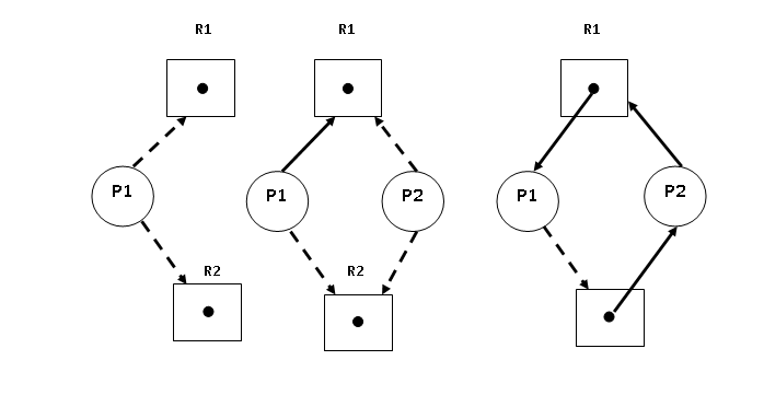
A new edge is introduced in the resource allocation graph called the Claim edge. means that it is a claim edge and shown as a dashed line in the resource allocation graph.
A claim edge shows “Future requests” or “Future Assignments” and converted to request edge and assignment edge respectively.
The request is granted only if converting request edge to an assignment edge does not lead to the formation of a cycle in the graph, if the allocation to will form a cycle that will lead the system to an unsafe state, then the process must wait till the resource is available.
Example:
\begin{aligned}
&P = \{P1, P2\}\\
&R = \{R_1, R_2\}
\end{aligned}| CLAIM EDGE | CONVERT TO REQUEST EDGE | CONVERT TO ASSIGNMENT EDGE |
 | YES | YES |
 | YES | YES |
 | NO (Make a cycle) | NO |
 | YES | NO (P1 using R1) |
Banker’s Algorithm
The algorithm works like a bank hence the name. Any new process must declare the maximum number of instance of each resource type that it needs. It must not exceed the total resource.
Before allocating the system must make sure that after allocation it is not leaving the system in the unsafe state.
The data structures used in banker’s algorithm where  is the number of processes and
  is the number of resource types is as follows,
- Available – number of available resources of each type of length
 .
. ![Available[j] = k](data:image/svg+xml;base64,PHN2ZyB4bWxucz0iaHR0cDovL3d3dy53My5vcmcvMjAwMC9zdmciIHdpZHRoPSIxMjUiIGhlaWdodD0iMTgiIHZpZXdCb3g9IjAgMCAxMjUgMTgiPjxyZWN0IHdpZHRoPSIxMDAlIiBoZWlnaHQ9IjEwMCUiIHN0eWxlPSJmaWxsOiNjZmQ0ZGI7ZmlsbC1vcGFjaXR5OiAwLjE7Ii8+PC9zdmc+ "Rendered by QuickLaTeX.com") means
means  instance of resource
  .
. - Max – It is
 matrix for maximum number instance of resources required by the process.
 ![Max[i][j] = k](data:image/svg+xml;base64,PHN2ZyB4bWxucz0iaHR0cDovL3d3dy53My5vcmcvMjAwMC9zdmciIHdpZHRoPSIxMDUiIGhlaWdodD0iMTgiIHZpZXdCb3g9IjAgMCAxMDUgMTgiPjxyZWN0IHdpZHRoPSIxMDAlIiBoZWlnaHQ9IjEwMCUiIHN0eWxlPSJmaWxsOiNjZmQ0ZGI7ZmlsbC1vcGFjaXR5OiAwLjE7Ii8+PC9zdmc+ "Rendered by QuickLaTeX.com") means
means  process requires instance of resource .
 - Allocation – it is also matrix for number of resources of each type allocated to each process.
![Allocation [i] [j] = k](data:image/svg+xml;base64,PHN2ZyB4bWxucz0iaHR0cDovL3d3dy53My5vcmcvMjAwMC9zdmciIHdpZHRoPSIxNDkiIGhlaWdodD0iMTgiIHZpZXdCb3g9IjAgMCAxNDkgMTgiPjxyZWN0IHdpZHRoPSIxMDAlIiBoZWlnaHQ9IjEwMCUiIHN0eWxlPSJmaWxsOiNjZmQ0ZGI7ZmlsbC1vcGFjaXR5OiAwLjE7Ii8+PC9zdmc+ "Rendered by QuickLaTeX.com") means process is allocated instances of resources of .
means process is allocated instances of resources of . - Need – it is matrix that remaining need for each process.
![Need[i] [k] = k](data:image/svg+xml;base64,PHN2ZyB4bWxucz0iaHR0cDovL3d3dy53My5vcmcvMjAwMC9zdmciIHdpZHRoPSIxMTAiIGhlaWdodD0iMTgiIHZpZXdCb3g9IjAgMCAxMTAgMTgiPjxyZWN0IHdpZHRoPSIxMDAlIiBoZWlnaHQ9IjEwMCUiIHN0eWxlPSJmaWxsOiNjZmQ0ZGI7ZmlsbC1vcGFjaXR5OiAwLjE7Ii8+PC9zdmc+ "Rendered by QuickLaTeX.com") means that the process need instance of resource type to finish its tasks.
means that the process need instance of resource type to finish its tasks.
![Available[j] = k](https://notesformsc.org/wp-content/ql-cache/quicklatex.com-37c53f881dbb832f41bbff70ce44ebed_l3.png "Rendered by QuickLaTeX.com") means
means  matrix for maximum number instance of resources required by the process.
 ![Max[i][j] = k](https://notesformsc.org/wp-content/ql-cache/quicklatex.com-c8e1b9ee717f504be9a548311ab63e9d_l3.png "Rendered by QuickLaTeX.com") means
means ![Allocation [i] [j] = k](https://notesformsc.org/wp-content/ql-cache/quicklatex.com-38caa8783fbbf2ee8808a398b076397f_l3.png "Rendered by QuickLaTeX.com") means process
means process ![Need[i] [k] = k](https://notesformsc.org/wp-content/ql-cache/quicklatex.com-03040c802283533ddf3783faaf78c735_l3.png "Rendered by QuickLaTeX.com") means that the process
means that the process Need[i] [j] = Max[i] [j] – Allocation[i] [j]Banker’s Algorithm Procedure
If  and
and  are two vectors, then
  only if
 ![X[i] \le Y[i]](https://notesformsc.org/wp-content/ql-cache/quicklatex.com-33fd94eb9fdd294afbde53bae71fbe70_l3.png "Rendered by QuickLaTeX.com") for all
for all  .
.
Conversely,  if
if ![Y[i] \le X[i]](https://notesformsc.org/wp-content/ql-cache/quicklatex.com-1e6d130a9600504559183fbc0b9617a3_l3.png "Rendered by QuickLaTeX.com") and
and  .
.
 means resource currently allocated to process and
  means additional resource required by process .
Safety Algorithm
1. Let "Work" and "Finish" be two vectors of length m and n respectively.
2. Initialize Work = Available and Finish[i] = false, for i = 0, 1, 2, ..., n-1.
3. Find an index ‘i’ such that
4. Finish[i] = false
5. Need(i) <= Work

If no such ‘i’ exists, then go to step 3.
6. Work = Work + Allocation (i)
7. Finish[i] = true
8. Go to step 2.

If Finish[i] = true for all i then the system is in safe state.
Order of the above algorithm is  .
.
Resource-Request Algorithm
This algorithm determines whether the request can be safely granted.
 is a request vector for process . If
 ![Request (i) [j] = k](https://notesformsc.org/wp-content/ql-cache/quicklatex.com-6f41bd4361246a64052bd81e692f666a_l3.png "Rendered by QuickLaTeX.com") , then process wants
, then process wants  instance of resource
 ![R[j]](https://notesformsc.org/wp-content/ql-cache/quicklatex.com-0dae2f5006f93e43e91be30f44a6085d_l3.png "Rendered by QuickLaTeX.com") . When a request for a resource is made, following activities take place
. When a request for a resource is made, following activities take place
- If
 , go to step 2, otherwise raise error because process has exceeded its maximum claim.
 - If
 , go to step 3. Otherwise, must wait, since the resources are not available.
 - Let system pretend that it has allocated the resources to as follows
 , go to step 2, otherwise raise error because process has exceeded its maximum claim.
 , go to step 3. Otherwise,
 \begin{aligned}
&Available = Available – Request (i)\\
&Allocation (i) = Allocation (i) + Request (i)\\
&Need (i) = Need (i) – Request (i)
\end{aligned}If the resulting resource-allocation state is in a safe state, the transaction is completed and process  gets the resource. If not, then must wait, and old resource-allocation state is restored.
Example:
\begin{aligned}
&P = \{P0, P1, P2, P3, P4\}\\\\
&R = \{A, B, C\}
\end{aligned}
Instances of Resources
A = 10, B = 5, C = 7
At  time following snapshot of system is captured.
| Allocation | Maximum | Available | |||||||
| A | B | C | A | B | C | A | B | C | |
 | 0 | 1 | 0 | 7 | 5 | 3 | 7 | 5 | 5 |
 | 2 | 0 | 0 | 3 | 2 | 2 | 5 | 3 | 2 |
 | 3 | 0 | 2 | 9 | 0 | 2 | 10 | 5 | 7 |
 | 2 | 1 | 1 | 2 | 2 | 2 | 7 | 4 | 3 |
 | 0 | 0 | 2 | 4 | 3 | 3 | 7 | 4 | 5 |
We know that 
| NEED Matrix | |||
| A | B | C | |
| 7 | 4 | 3 |
| 1 | 2 | 2 |
| 6 | 0 | 0 |
| 0 | 1 | 1 |
| 4 | 3 | 1 |
Check if the System is in Safe State
Iteration 1
Step 1:
\begin{aligned}
&Need (i) <= Available, \hspace{3px}if \hspace{3px} True then,\\\\
&Need (0) > Available => (7, 4, 3) > (3, 3, 2)\\\\
&Need (1) < Available => (1, 2, 2) < (3, 3, 2)
\end{aligned}
Step 2:
\begin{aligned}
&Work = Work + Allocation (i)\\\\
&Work = (3, 3, 2) + (2, 0, 0) = (5, 3, 2)\\\\
&
\end{aligned}
Step 3:
\begin{aligned}
&Add \hspace{3px}P_1 \hspace{3px}to \hspace{3px}Safety \hspace{3px}Sequence\\\\
&Safety \hspace{3px} sequence = \{P_1\}
\end{aligned}
Iteration 2
Step 1:
\begin{aligned}
&Need (i) <= Available, \hspace{3px} if  \hspace{3px} True  \hspace{3px} then,\\\\
&Need (2) > Available => (6, 0, 0) > (5, 3, 2)\\\\
&Need (3) < Available => (0, 1, 1) < (5, 3, 2)\\\\
\end{aligned}
Step 2:
\begin{aligned}
&Work = Work + Allocation (i)\\\\
&Work = (5, 3, 2) + (2, 1, 1) = (7, 4, 3)\\\\
\end{aligned}
Step 3:
\begin{aligned}
&Add \hspace{3px} P_1 \hspace{3px} to \hspace{3px} Safety \hspace{3px}Sequence\\\\
&Safety \hspace{3px}sequence = \{P_1, P_3\}
\end{aligned}
Iteration 3
Step 1:
\begin{aligned}
&Need (i) <= Available, \hspace{3px} if \hspace{3px}True \hspace{3px}then,\\\\
&Need (4) <= Available => (4, 3, 1) < (7, 4, 3)
\end{aligned}
Step 2:
\begin{aligned}
&Work = Work + Allocation (i)\\\\
&Work = (7, 4, 3) + (0, 0, 2) = (7, 4, 5)
\end{aligned}
Step 3:
\begin{aligned}
&Add \hspace{3px}P_1 \hspace{3px}to \hspace{3px}Safety \hspace{3px}Sequence\\\\
&Safety \hspace{3px}sequence = \{P_1, P_3, P_4\}
\end{aligned}
Iteration 4
Step 1:
\begin{aligned}
&Need (i) <= Available, \hspace{4px} if \hspace{4px} True  \hspace{4px} then,\\\\
&Need (0) <= Available => (7, 4, 3) < (7, 4, 5)\\\\
\end{aligned}
Step 2:
\begin{aligned}
&Work = Work + Allocation (i)\\\\
&Work = (7, 4, 5) + (0, 1, 0) = (7, 5, 5)
\end{aligned}
Step 3:
\begin{aligned}
&Add \hspace{3px}P_1 \hspace{3px}to \hspace{3px}safety \hspace{3px}sequence\\\\
&Safety \hspace{3px}sequence = {P1, P3, P4, P0}
\end{aligned}
Iteration 5
Step 1:
\begin{aligned}
&Need (i) <= Available, \hspace{3px}if \hspace{3px}True \hspace{3px}then,\\\\
&Need (2) <= Available => (6, 0, 0) < (7, 5, 5)
\end{aligned}
Step 2:
\begin{aligned}
&Work = Work + Allocation (i)\\\\
&Work = (7, 5, 5) + (3, 0, 2) = (10, 5, 7)
\end{aligned}
Step 3:
\begin{aligned}
&Add \hspace{3px}P_1 \hspace{3px}safety \hspace{3px}sequence\\\\
&Safety \hspace{3px}sequence = \{P_1, P_3, P_4, P_0, P_2\}
\end{aligned}
Handling a Request
Suppose process requested resource  which is less than the available resources
  .
.
Request (i) <= Available => (1, 0, 2) < (3, 3, 2)
The system will pretend that the resource is allocated successfully but will run the Safety Algorithm demonstrated above and verify if whether allocation to will leave the system in an UNSAFE state.
Example:
Suppose requested for  , then we find that
  Adjust the following
\begin{aligned}
&Available:= Available - Request;\\\\
&Allocation; =Allocation +Request;;\\\\
&Need; =Need- Request;
\end{aligned}| Allocation | Maximum | Available | |||||||
| A | B | C | A | B | C | A | B | C | |
| 0 | 3 | 0 | 7 | 5 | 3 | 3,7 | 1,5 | 2,5 |
| 2 | 0 | 0 | 3 | 2 | 2 | 5 | 1 | 2 |
| 3 | 0 | 2 | 9 | 0 | 2 | |||
| 2 | 1 | 1 | 2 | 2 | 2 | 7 | 2 | 3 |
| 0 | 0 | 2 | 4 | 3 | 3 | 7 | 2 | 5 |
We then run the Safety Algorithm
| NEED Matrix | |||
| A | B | C | |
| 7 | 2 | 3 |
| 1 | 2 | 2 |
| 6 | 0 | 0 |
| 0 | 1 | 1 |
| 4 | 3 | 1 |
Iteration 1
Step 1:
\begin{aligned}
&Need (i) <= Available, \hspace{3px}if \hspace{3px}True \hspace{3px}then,\\\\
&Need (1) <= Available => (1, 2, 2) < (3, 1, 2)\\\\
\end{aligned}
Step 2:
\begin{aligned}
&Work = Work + Allocation (i)\\\\
&Work = (3, 1, 2) + (2, 0, 0) = (5, 1, 2)
\end{aligned}
Step 3:
\begin{aligned}
&Add \hspace{3px}P_1 \hspace{3px}to \hspace{3px} safety \hspace{3px}sequence\\\\
&Safety \hspace{3px} sequence = {P1}
\end{aligned}
Iteration 2
Step 1:
\begin{aligned}
&Need (i) <= Available, \hspace{3px} if \hspace{3px}True \hspace{3px}then,\\\\
&Need (2) > Available => (6, 0, 0) > (5, 1, 2)\\\\
&Need (3) <= Available => (0, 1, 1) < (5, 1, 2)
\end{aligned}
Step 2:
\begin{aligned}
&Work = Work + Allocation (i)\\\\
&Work = (5, 1, 2) + (2, 1, 1) = (7, 2, 3)
\end{aligned}
Step 3:
\begin{aligned}
&Add \hspace{3px}P_3 \hspace{3px} to \hspace{3px} safety \hspace{3px} sequence\\\\
&Safety \hspace {3px} sequence = \{P_1, P_3\}
\end{aligned}
Iteration 3
Step 1:
\begin{aligned}
&Need (i) <= Available, \hspace{3px}if \hspace{3px}True \hspace{3px} then,\\\\
&Need (4) <= Available => (4, 3, 1) < (7, 2, 3)\\\\\end{aligned}
Step 2:
\begin{aligned}
&Work = Work + Allocation (i)\\\\
&Work = (7, 2, 3) + (0, 0, 2) = ( 7, 2, 5 )
\end{aligned}
Step 3:
\begin{aligned}
&Add \hspace{3px} P_1 \hspace{3px} to \hspace{3px} safety \hspace{3px} sequence\\\\
&Safety \hspace{3px}sequence = \{P_1, P_3, P_4 = not \hspace{3px}  safe\}
\end{aligned}
References
- Abraham Silberschatz, Peter B. Galvin, Greg Gagne, A Silberschatz. 2012. Operating System Concepts, 9th Edition. Wiley.
Operating Systems Notes – Concepts, Examples, and Exam-Ready Revision
Operating Systems are a core subject in Computer Science and Information Technology (IT) curricula, as well as in competitive examinations such as GATE, UGC NET, and university semester exams.
On this page, you will find structured resources to learn operating systems concepts, along with clear explanations, examples and exam-ready revision notes.
What Will You Learn
On this page you will find:
- Core Operating Systems concepts explained clearly and systematically
- Exam-oriented explanations supported with relevant examples
- MCQ-based practice posts to test your understanding
- Detailed articles along with exam-ready revision PDFs
This Page is for:
- Computer science and IT students
- GATE and other competitive exam aspirants
- University exam preparation
- Self learners who want to revise data structures knowledge.
Topic Sections
Find Data Structures topics here.
(1) Introduction to Operating Systems
(2) Operating Systems Structures
(3) Process Concepts
- OS Process Concepts
- OS Process States
- Inter-Process Communications
(4) Threads & Concurrency
- Multi-Threaded Programming
- Pthreads
- Win32 Threads
- Java Threads
- Concurrency
(5) CPU Scheduling
- Types of Schedulers
- Process Scheduling Criteria
- First Come, First Served (FCFS)
- Shortest Job First ( SJF )
- Round Robin
- Priority Scheduling
- Shortest Remaining Time First (SRTF)
- Multilevel Queue
- SJF Tabular Method
- FCFS Tabular Method
(6) Process Synchronization
- Critical Section Problem
- Critical Section Solution
- Bounded-Buffer Problem
(7) Deadlocks
(8) Main Memory Management
- Memory Mapping Schemes
- Logical vs. Physical Memory Address
- Dynamic Loading And Linking
- OS Swapping Processes
- Contagious Memory Allocation
(9) Virtual Memory
- Paging
- Page Table
- Page Replacement Techniques
- Segmentation