The usual method of computing average time, average wait time, turnaround time and average turnaround time for processes is to make a Gantt Chart and then compute these times. In this article, we explore another way to compute the average turnaround time and average wait time for processes based on the same logic given by the specific algorithm.
CPU Scheduling Algorithms
In the previous article, you learnt how tabular method computer the turnaround time and wait time for SJF algorithm. The popular CPU scheduling algorithms are as follows
- First Come, First Serve
- Shortest Job First
- Priority Scheduling
- Round Robin
This article, we use tabular method on FCFS (first come, first serve). Throughout the post, we will use the same example to compute the times using FCFS. Consider the following processes.

We will compute the average turnaround time and average wait time for the processes using the tabular method.
First Come, First Serve
At first, make a table as follows, with processes ordered in the way they arrive in the queue.

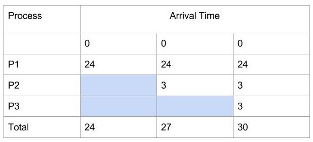
The first column is for processes in the ready queue and listed in the order as they arrive. The arrival of all three processes is 0.
- Fill the first row with burst time of process P1.
- Fill the second row with burst time of process P2 because it starts after P1.
- Similarly, fill the burst time of P3 in the third row last column because P3 start after P2 process.
- Each column is Turnaround time for each process in the queue.
\begin{aligned}
&Average \hspace{3px}Turnaround \hspace{3px} Time = \frac{(24 + 27 + 30)}{3 }= \frac{81}{3} = 27 \hspace{3px} ms
\end{aligned}
Note: waiting time of the first process is always 0.
To compute the average waiting time of each process, add all the value in row Total, except the last column and divide by a number of processes.
\begin{aligned}
&Average \hspace{3px}Waiting \hspace{3px}Time = \frac{(0 + 24 + 27)}{3 }= \frac{51}{3} = 17 \hspace{3px}ms
\end{aligned}
First Come, First Serve with Change in Order
Suppose we change the order of execution. Does that change the average waiting time and turnaround time of the processes scheduled using the FCFS, let’s find out the answer.
\begin{aligned}
&Average \hspace{3px}Turnaround \hspace{3px}Time = \frac{(3 + 6 + 30)}{ 3 }= 13 \hspace{3px}ms \\\\
&Average \hspace{3px}Waiting \hspace{3px}Time = \frac{(0 + 3 + 6)}{3 }= 3 \hspace{3px}ms
\end{aligned}
In the above example, process P3 is the first, process P2 is second and process P4 is the third in that order. We already know the wait time of the process P3 = 0 because it is the first process to arrive in the queue.
For turnaround time take the total of row “Total” and divide by 3 will give you the answer and for the average waiting time, the sum of first two columns of the row “Total” divided by 3 will give you the answer.
First Come, First Serve with different Arrival Times
Consider another example, here process arrive at the ready queue with different times.

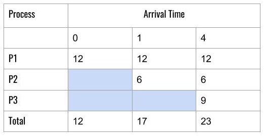
To compute the average turnaround time and average waiting time using the tabular method. Draw following table but this time we have different arrival times for each process.

To calculate the individual Turnaround time for each process, we need to take the column total for minus the arrival time in the same column.
For example
\begin{aligned}
&In \hspace{3px}the  \hspace{3px}first \hspace{3px}column,\\&we  \hspace{3px}have  \hspace{3px}a  \hspace{3px}Total = 12 - 0  \hspace{3px}(Arrival  \hspace{3px}Time) \\&= 12 \hspace{3px}( Turnaround  \hspace{3px}time  \hspace{3px}for  \hspace{3px}P1)\\\\
&In  \hspace{3px}the  \hspace{3px}second  \hspace{3px}column, \\&we \hspace{3px} have  \hspace{3px}a  \hspace{3px}Total = 18 - 1( Arrival  \hspace{3px})\\& = 17 ( Turnaround  \hspace{3px}time  \hspace{3px}for P2)\\\\
&Average  \hspace{3px}Turnaround  \hspace{3px}time = \frac{(12 + 17 + 23)}{3} = \frac{52}{3} = 17.33  \hspace{3px}ms.
\end{aligned}
To compute the waiting time of each process, take each column total – next process arrival time and you get the results.
For example
\begin{aligned}
&waiting \hspace{3px}time \hspace{3px}for \hspace{3px}P1 = 0\\\\
&waiting \hspace{3px}time\hspace{3px} for\hspace{3px} P2 = 12 - 1 = 11\\\\
&time \hspace{3px}for \hspace{3px}P3 = 18 - 4 = 14\\\\
&Average \hspace{3px}Waiting \hspace{3px}Time = \frac{(0 + 11 + 14)}{3} = \frac{25}{3} = 8.33 \hspace{3px}ms
\end{aligned}
Conclusion
The tabular method employs the same method as performing calculations using Gantt Char but if the number of processes and other data becomes too complex then you may tend to make mistakes. Then using the Tabular method simplifies the calculations.
In the next post in this series, we will see more complex examples and how they can be tackled using this method of calculation.
References
- Abraham Silberschatz, Peter B. Galvin, Greg Gagne, A Silberschatz. 2012. Operating System Concepts, 9th Edition. Wiley.
