Functional Dependencies in DBMS: Use of FD in Table Design
A Functional dependency is used to describe the relationship between attributes of a relation. In other words, it explains how one or more columns of a database table determine other columns. In this article, we will discuss, the use of functional dependencies in table design and uses of functional dependencies.
Let \Large X be a set of attributes, and \Large Y be another set of attributes.
If two rows of a relation have the same values for the attributes in \Large X, then they must have the same values for the attributes in \Large Y. This is known as the uniqueness property, and every functional dependency satisfies this property.
A functional dependency between \Large X and \Large Y is denoted as \Large X \rightarrow Y where \Large X is called the determinant and \Large Y is the dependent attribute set.
Example of Functional Dependency (FD)
Consider the following database table.
| StudentID | StudentName | Department |
|---|---|---|
| 20 | Peter Pan | Mathematics |
| 21 | Ravi Kumar | Physics |
| 22 | Kiran Joshi | Chemistry |
For each StudentID, there is only one StudentName. If two rows have same StudentID, then their StudentName must be same.
Similarly, for each StudentID there is exactly one Department. If two rows have same StudentID, then the deparment must contain same value.
This satisfies the uniqueness property of functional dependency.
Functional Dependencies in the Student Table
\Large StudentID \rightarrow StudentName\\StudentID \rightarrow Department
StudentName and Department are functionally dependent on StudentID. The StudentID is the determinant.
What Happens When There is no Functional Dependency
Consider another table with attributes – StudentID and CourseID.
| StudentID | CourseID |
|---|---|
| 21 | CS101 |
| 21 | CS102 |
| 22 | CS104 |
The table shows that some students are associated with more than one CourseID.
Therefore, StudentID does not uniquely determine CourseID, and the uniqueness property is not satisfied for this relationship.
This means the functional dependency
\Large StudentID \rightarrow CourseID
does not hold.
- StudentID does not uniquely determines CourseID.
- Student can be associated with many Courses.
A functional dependency exists only when the left-hand side attributes (determinants) uniquely determine the right-hand side attributes (dependent).
If one value of set \Large X, is mapped to multiple values of \Large Y, then \Large X \rightarrow Y is not functional dependency.
In the real world, a student can enroll in multiple courses. Although there is a meaningful relationship between students and courses, it is not a functional dependency.
While designing a database, the learner must carefully distinguish between:
- Meaningful relationships, and
- Functional dependencies, which require uniqueness.
Only relationships that satisfy the uniqueness property can be modeled as functional dependencies.
Composite Functional Dependency
Consider the following Grade Table.
| StudentID | CourseID | Grade |
|---|---|---|
| 21 | CS101 | A |
| 22 | CS104 | B |
| 23 | CS102 | B |
Step 1: Check for Individual Attributes
The StudentID alone cannot uniquely identify a student’s Grade. Students may obtain same grade for different courses.
Similarly, the CourseID alone cannot uniquely identify the grade of a student. Different student may get same grade for same course. There is no uniqueness.
Step 2: Check for Combination of Attributes
Consider the following combination:
\Large \{StudentID, CourseID\}Now we can uniquely identify a grade. Therefore, the functional dependency
\Large \{StudentID, CourseID\} \to Gradeholds.
This is called a composite functional dependency because the determinant consists of more than one attribute. In such a dependency, the left-hand side of the functional dependency is called a composite determinant.
Why Functional Dependencies Matter Before Normalization
Normalization is a formal process that restructures tables based on functional dependencies (FDs). Forms such as 2NF, 3NF, and BCNF are defined entirely in terms of FDs.
Therefore, normalization cannot begin until functional dependencies are identified and analyzed.
Role of Functional Dependencies (FDs)
Before normalization, functional dependencies are used to:
- Identify candidate keys
- Detect redundancy
- Explain insertion, update, and deletion anomalies
Each of these tasks relies on formal dependency rules, not intuition
Identifying Keys
Functional dependencies are used to find the candidate keys of a table. A candidate key is a set of attributes \Large K that determines all other attributes of the table, and no proper subset of \Large K can do the same.
To find candidate keys, we use a procedure called attribute closure.
The closure of attribute set \Large K written as \Large K^+
- is the set of all attributes
- that can be functionally determined from \Large K
- using the given functional dependencies.
The attribute closure of a set of attributes finds all attributes that are functionally determined by that set using the given functional dependencies. If the closure of a set K contains all attributes of the table and no proper subset of has this property, then is a candidate key.
Formally, if
- \Large K^+ contains all attributes of the relation.
- No other proper subset can this property,
\Large K is the candidate key.
Example – Find the Candidate key for Student Table.
Consider a Student table with four attributes: StudentID, CourseID, StudentName, and Grade.
We usually begin by computing the closure of single attributes.
\Large \{StudentID\}^+ = \{ StudentID\}The attribute itself is always included in its closure.
\Large StudentID \to StudentNameUsing the functional dependency StudentID → StudentName, we add StudentName to the closure.
\Large \{StudentID\}^+ = \{StudentID, StudentName\}StudentName is part of closure
\Large StudentID \to GradeThere is no functional dependency StudentID → Grade, so Grade cannot be added to the closure.
Let us check closure for CourseID.
\Large \{CourseID\}^+ = \{CourseID \}Initial value added to closure.
\Large CourseID \to GradeThe above is not a dependency.
\Large \{CourseID\}^+is not candidate set of keys.
Check closure of all attributes.
\Large \{StudentID, CourseID, Grade\}^+ = \{StudentID, CourseID, Grade\}Initial value added to closure.
This is the candidate key which functionally determine all attributes in the table.
Can we minimize it ?
Yes, the Grade can be determined by \Large \{StudentID, CourseID\}, but \Large StudentID or \Large CourseID cannot be determined alone.
Conclusion
The candidate key for the student table is the set \Large {StudentID, CourseID} because it determine all the attributes in the table.
\Large \{StudentID, CourseID\} \to Grade.
\Large\{StudentID, CourseID\} \to StudentID.
\Large \{StudentID, CourseID\} \to CourseID.
Another use of FD is to find the redundancy.
FD and Redundancy
From the above discussion, it clear that a functional dependency is either determinant or dependent in an optimized table. Any table attribute that it dependent on non-key attribute is likely to have duplicate values.
Therefore, functional dependencies reveal such attributes that are dependent on non-key attributes.
Consider the Student table with three attributes – StudentID, DepartmentID, and DeptName.
| StudentID | DepartmentID | DeptName |
|---|---|---|
| 20 | D101 | Mathematics |
| 21 | F102 | Physics |
| 22 | F102 | Physics |
The functional dependencies are:
\Large StudentID \to DepartmentID \\
DepartmentID \to DeptName
DeptName is not functionally dependent on StudentID.
The nature of functional dependency is Transitive.
\Large StudentID \to DepartmentID \to DeptName
We always want to remove the Transitive dependencies.
In these case, each student will not have exactly one value for Department name, but contains multiple redundant values.
Describe The Insert, Update and Deletion Anomalies
Here is a list of problems due to redundancies.
Insert anomalies – Unless student exists department id cannot be assigned , so a new department is not created if we don’t have a student. This is Insert anomalies.
Update anomalies – The table shows two students from same department – Physics. If we want to rename the Physics to something else, say Quantum Physics. We must change all the records where department name is Physics. This is update anomalies.
Deletion anomalies – If we delete the record for Student with id 20, then the department cease to exist. This is deletion anomalies.
Let us take another example.
The following Student table have four attributes – StudentID, CourseID, StudentName, and Grade.
| StudentID | CourseID | StudentName | Grade |
|---|---|---|---|
| 20 | M201 | Peter Pan | C |
| 20 | P101 | Peter Pan | A |
| 21 | X106 | Ravi Kumar | B |
| 21 | A44 | Ravi Kumar | A |
Let us identify the functional dependencies from the table.
\Large StudentID \to StudentName\\
\{StudentID, CourseID\} \to Grade
Clearly, the primary key is \Large \{StudentID, CourseID\}.
However, StudentName is only dependent on StudentID. This is Partial Dependency.
Conclusion
The solution to example 1 and example are same:
Example 1 – In case of transitive dependency, split the table into two.
| StudentID | DepartmentID |
|---|---|
| 21 | F102 |
| 22 | F102 |
| DepartmentID | DeptName |
|---|---|
| F102 | Physics |
| D101 | Mathematics |
The Student table has multiple same values, this is not redundancy. The StudentID is unique key and it identity the row in Student table uniquely.
The department table is totally unique because each department id has exactly one department.
Example 2 – In the case of partial dependency, you have to split the table again.
| StudentID | StudentName |
|---|---|
| 20 | Peter Pan |
| 21 | Ravi Kumar |
| StudentID | CourseID | Grade |
|---|---|---|
| 20 | M201 | C |
| 21 | A44 | A |
In the second example, StudentID or CourseID, alone cannot determine the Grade. Here are the functional dependencies from both tables.
Student Table
\Large StudentID \to StudentName
Grade Table
\Large \{StudentID, CourseID\} \to GradeThe separate tables ensure that each row is unique and do not have redundant data.
You have seen two different types of functional dependencies. In the next section, we shall explore all types of functional dependencies.
Types of Functional Dependencies (Using Tables)
The functional dependencies are classified based on attribute dependencies. Its the relationship between determinant attributes and dependent attributes.
Trivial Functional Dependency
A functional dependency \Large X \to Y from a set of attributes \Large X to a set of dependent attributes \Large Y is trivial if \Large Yis a subset of \Large X.
In other words, all the attributes of \Large Y are already in \Large X.
\Large X \to Y, is \hspace{4px} trivial \hspace{4px} if \hspace{4px} Y \subseteq XExample – Trivial Dependency
| StudentID | CourseID |
|---|---|
| 21 | A44 |
| 22 | P203 |
Observe that the key is \{StudentID, CourseID\} because StudentID or CourseID alone cannot be key.
Given the key, the following functional dependencies are Trivial.
\Large \{StudentID, CourseID\} \to StudentID\\
\{StudentID, CourseID\} \to CourseID
Axiom Used in Trivial Dependency
The Armstrong’s axiom used in trivial functional dependency is called the Reflexivity rule.
\Large FD: A \to A, \hspace{5px} because \hspace{5px} A \subseteq ANon-Trivial Functional Dependency
A functional dependency \Large X \to Yfrom a set of attributes \Large X to a set of dependent attribute \Large Y is Non-Trivial if \Large Y is non a subset of \Large X.
\Large X \to Y \hspace{4px} is \hspace{4px} Non-Trivial \hspace{5px} if \hspace{4px}Y \nsubseteq XExample – Non Trivial Dependency
| StudentID | StudentName |
|---|---|
| 20 | Peter Pan |
| 21 | Ravi Kumar |
The StudentID is the key and StudentName is dependent attribute. Also,
\Large StudentID \to StudentName,\\
\{StudentName\} \nsubseteq \{StudentID\}
The StudentName is not a subset or equal to set StudentID.
Axioms User in Non-Trivial Dependency
The non-trivial dependency is derived from other Armstrong’s axioms.
Suppose we have a functional dependency, \Large A \to \{B, C\} is called a Union Rule. The functional dependency can be decomposed into:
\Large FD: A \to \{B, C\} = \{A \to B\} \hspace{4px} and \hspace{5px} \{A \to C\}Completely Non-Trivial Functional Dependency
A functional dependency \Large ( X \to Y ) is a completely non-trivial dependency for two sets of attributes \Large X and \Large Y if:
\Large X \cap Y = \empty
In a completely non-trivial dependency, the sets \Large X and \Large Y are disjoint, and their intersection is a null or empty set.
Example – Completely Non-Trivial Dependency
| StudentID | DeptName |
|---|---|
| 20 | Mathematics |
| 21 | Physics |
| 21 | Computer Science |
Notes that \Large StudentID \cup DeptName are disjoint sets.
However, the functional dependency holds.
\Large StudentID \to DeptName
The functional dependency is correct, but each student can have more than one department. The student with ID 21 has two separate departments. This will cause redundancy in the table. You must normalize the table in such cases.
Full Functional Dependency
A dependency from \Large X \to Y is Full dependency if:
- \Large Y is dependent on all attributes of \Large X.
- No proper subset of \Large Xcan determine \Large Y.
Symbolically,
\Large \begin{aligned}
&X \to Y \hspace{5px} is  \hspace{5px} a \hspace{5px} Full \hspace{5px}Functional \hspace{5px} Dependency \hspace{5px} if:\\
&1. \hspace{3px}Y \not \subset X\\
&2. \hspace{3px} X' \not \to Y, \hspace{5px} where \hspace{5px} X' \subset X
\end{aligned}
Example – Full Functional Dependency
In this example, consider Student table with StudentID, CourseID and Grade.
| StudentID | CourseID | Grade |
|---|---|---|
| 20 | M203 | C |
| 21 | A44 | A |
This is a full functional dependency where Grade is dependent on key \Large \{StudentID, CourseID\}.
\Large \{StudentID, CourseID\} \to GradeNow to validate, that this is full functional dependecy, we must check the conditions.
- \Large Y is not a subset of \Large X.
\Large \{StudentID, CourseID\} \nsubseteq Grade2. \Large X' cannot determine \Large Y, where \Large X' is proper subsets of \Large X.
\Large StudentID \not \to Grade\\
CourseID \not \to Grade
Hence, it is proved that the functional dependency is a full functional dependency.
Partial Functional Dependency
A functional dependency \Large X \to Y is a Partial functional dependency if:
- \Large X is composite. In other words, \Large X has more than one attributes.
- \Large Y depends only on part of \Large X.
Example – Partial Functional Dependency
Consider the student table.
| StudentID | CourseID | StudentName |
|---|---|---|
| 20 | CS101 | Peter Pan |
| 21 | A44 | Ravi Kumar |
We have two functional dependencies in the above table.
\Large \{StudentID, CourseID\} \to StudentName\\
StudentID \to StudentName
Let us check the conditions for partial dependency.
- \Large X is composite. This condition is true because \Large \{StudentID, CourseID\} uniquely determine all the attributes in the student table.
- \Large Y depends on part of \Large X. This is also true, because StudentName is dependent only on StudentID, and not on CourseID of composite key \Large \{StudentID, CourseID\}.
The partial dependency causes redundancy and violates the second normal form \Large (2NF). You will learn \Large (2NF) in future posts.
Transitive Functional Dependency
A functional dependency \Large X \to Y is Transitive if there exists another dependency \Large Y \to Z such that \Large X \to Z also exists. The \Large X \to Z is also a function dependency.
\Large \to Y \hspace{5px} is \hspace{5px} Transitive \hspace{5px} if:\\

X \to Y \hspace{5px} and \hspace{5px} Y \to Z \hspace{5px} implies \hspace{5px} X \to Z
Example – Transitive Functional Dependency
Consider the following Employee table.
| EmployeeID | DeptID | DeptAddress |
|---|---|---|
| 4331 | D12 | New Delhi |
| 4332 | D13 | Chennai |
| 4333 | D14 | Mumbai |
| 4334 | D14 | Mumbai |
We see two functional dependencies in the Employee table.
\Large EmployeeID \to DeptID\\
DeptID \to DeptAddress
Since, EmployeeID determines DeptID and DeptID determines DeptAddress.
A transitive functional dependency. exists between ExployeeID and DeptAddress.
\Large ExployeeID \to DeptAddress
A transitive dependency contains redundant data.
If you look at the Employee table, the department address Mumbai is repeated every time when an employee has department ID of D14. In these cases, splitting the table is the best solution.
Now, you know everything about Functional dependencies, let us summarize what you learned.
Summary
These are important points to remember for exams.
Uses Of Functional Dependencies (Concept Overview for Revision)
| Purpose of FDs | Explanation |
|---|---|
| Identify Keys | Determine candidate keys and primary keys using attribute closure. |
| Detect Redundancy | Reveal the duplicate storage of same information across many rows. |
| Explain Anomalies | Identify Insertion, Update and Deletion anomalies. |
| Guide the Normalization Process | Decompose relations into normal forms. |
| Improve Table Design | Ensure minimum duplicates and improve logical data organizations. |
Types of Functional Dependencies
| Dependency Type | Concept |
|---|---|
| Trivial Functional Dependency | Dependent attribute is already part of Determining attributes. |
| Non-Trivial Functional Dependency | Dependent attribute is NOT part of Determining attributes. |
| Completely Non-Trivial Functional Dependency | Dependent and Determinant attributes have nothing in common. |
| Full Functional Dependency | The Dependent attributes depend on the entire set of Determining attributes and not on any proper subset of Determining attributes. |
| Partial Functional Dependency | Depending attributes depends only on subset of Determining Attributes. |
| Transitive Functional Dependencies | Dependent attributes indirectly dependent on the Determining attributes. |
Data Models in DBMS: Data Abstraction, Levels, and Types
Data models are fundamental concepts in DBMS that help in database design. They enable communication between database designers, application developers, and end-users.
A Data model defines how data is structured, organized, and represented in a database system. The topic is foundation for database design, and it is an important part of the DBMS syllabus.
In this post, we will explain the concepts of data models, data model levels, and understand different types of data models. This topic is frequently asked in university examinations and competitive examinations like GATE, etc.
Before we begin, let’s understand data abstraction.
What is Data Abstraction?
The data abstraction means only exposing the essential data to the users and hiding the implementation details. We don’t show the storage details.
The purpose of data abstraction is:
- Provide security and data protection.
- Data independence
- Reduce complexity
- Easy maintenance
Provide security and data protection
The data abstraction keeps different access for different users. It hides the sensitive data from normal users. Users cannot access the data directly without authentication.
Data Independence
Data abstraction is independent of physical storage. A change in storage structure such as files, indexes, etc., will not affect the application level data. They are independent of each other.
Reduce Complexity
Keeping separate layers of data and hiding their implementation details reduces complexity. Users only see what is necessary for them.
For example, users interact with logical tables, without knowing the storage details.
Easy Maintenance
We already mentioned that data abstraction is data independence. Each layer is separate and does not affect the higher layer. We can repair physical disks, without affecting user’s access to tables.
This makes the maintenance process easy.
What is Data Model ?
The data model is the blueprint that defines the structure of the database. It is the foundation of database design. The structure of the database includes its
- Data types
- Relationships and
- Database constraints.
The data model is designed and organized to solve the data requirements of a specific application or specific domain, not all applications. It only supports a specific problem area.
A key feature of a data model is the data organization, which defines how data and relationships are structured in the database.4
In next section, you will learn more about different levels of data models.
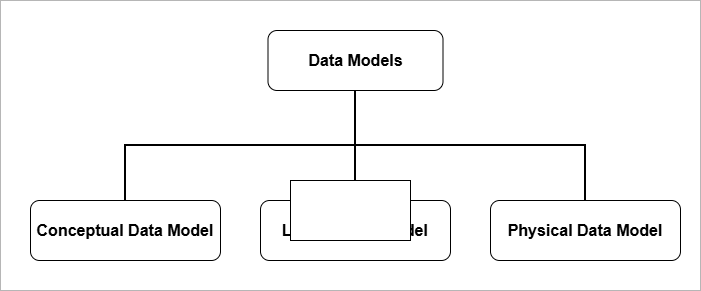
Three Levels of Data Models
It is necessary to separate the data models into three distinct levels of modeling. Each level of data model collects different data and implements them differently.
- Conceptual Data Model
- Logical Data Model
- Physical Data Model
Conceptual Data Model
A conceptual data model is a high-level model that provides
- an overall logical view of the database that is easy for non-technical stakeholders to understand. It consists of real-world concepts and business logic.
- It tells us what kind of data is required, independent of database or storage details. It reveals business requirements such as entities and their relationships.
- The conceptual layer enables communication between the database designer, application developer, and end users. All of them collaborate to build a database system that solves a specific problem.
- The conceptual level serves as a blueprint for both the logical data model and the physical data model.
In relational database systems, conceptual modeling involves creating an Entity–Relationship (E–R) model or an object model. Its main purpose is to answer two questions:
- What data is required?
- How should the data be organized ?
At the conceptual data model level, data is represented as entities and their relationships, where an entity represents a real-world object.
Object modeling uses UML (Unified Modeling Language), use-case diagrams, etc., to model user interaction with the database through a software system.
After conceptual data model is completed, the next step is to design a logical data model.
Logical Data Model
The main purpose of logical data model is to answer one question, “How is the data organized?”.
The logical data model is used to design database relations and their relationships based on the conceptual model, without specifying physical storage details.
The logical (relational) model is the core of database systems (DBMS) because it defines how data is organized, related, and accessed.
The E–R diagram from the conceptual model is translated into a relational model.
Data is organized into tables (relations) that contain columns (attributes), keys, and relationships.
The next step after the logical data model is to implement the database on disks and storage devices
Physical Data Model
The physical data model defines the files, storage structures, and other storage-level details of the database. This level answers the question:
“How is the data stored?”
The physical data model includes:
- File system
- Indexes
- Storage allocation
- Records placements
- Access paths
The storage level details are hidden from the common users of the database system.
- At storage level, faster searches is achieved through indexes,
- Disk performance is enhanced using disk access algorithms.
- Storage security ensures protection of servers from damage, power failures, and theft.
Different types of models correspond to different levels of data modeling. The conceptual level captures concepts in the form of entities and relationships. The logical level defines how data is organized. The physical level selects efficient storage structures.
In the next section, we discuss different types of data models.
Types of Data Models (Logical)
Logical models represent different ways of organizing data and relationships. The main types are:
- Hierarchical model
- Network model
- Relational model
Hierarchical Data Model
The hierarchical data model stores data in a tree-based structure.
- The tree-like structure helps represent natural hierarchies.
- A strict parent–child relationship ensures data integrity.
- The tree-based structure is simple and predictable.
- The data retrieval is faster if you know the path as it is fixed.
- Access begins from the root node, which means nodes closer to the root are accessed more quickly.
Components of a Hierarchical Data Model
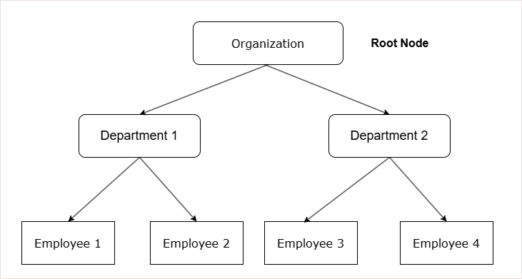
1. Tree Structure
The hierarchical data model is based on a parent–child relationship.
- Each parent can contain multiple child nodes.
- Each child node can have only one parent.
2. Nodes
Data is organized into a logical units called nodes.
- Each node represents a specific type of record.
3. Root Node
The top of the tree contains a single node called the root node.
- The root node has no parent.
- It is the starting point for data access and navigation.
4. Leaf Nodes
The lowest-level nodes in the tree are called leaf nodes.
- A leaf node has no children.
* Data organization begins from the root node.
* It follows strict parent–child relationships.
* Each child has only one parent, while each parent can have multiple children.
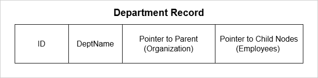
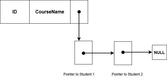
How records are stored in Hierarchical model?
The records in hierarchical model has many fields, including the following;
- A pointer to parent node, except root node.
- Pointers to many child nodes
Data retrieval in a hierarchical data model requires traversing the nodes from the root node to the specific record.
- You can only traverse records starting from the root node.
- Retrieval is top-down and one-way.
In a hierarchical data model, data retrieval is one-way, typically from parent to child, following a fixed top-down path.
Limitations of Hierarchical Model
The hierarchical data model has several limitations:
- The structure is rigid and suitable only for one-to-one or one-to-many parent-to-child relationships.
- The search path is fixed and always begins from the root node.
- There is no support for many-to-many relationships.
An improved alternative to the hierarchical model is the network model.
In the next section, you will learn about the network model.
Network Data Model
The network data model has a graph-like structure.
- There is no root node, unlike the hierarchical model.
- In this model, a child node can have multiple parents, and a parent can have multiple children.
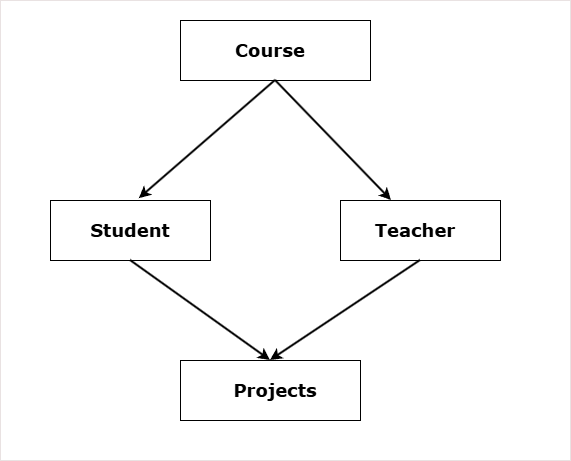
The diagram shows a network data model for school where:
- One course has one or many students.
- One course has one or many teachers.
- One student has one or more projects to complete.
- One teacher guide students on one or many projects.
Components of Network Data Model
The main components of network data model are:
- Record Type
- Data Item (attribute)
- Set Type
- Owner Records
- Member Records
- Links (Pointers)
Record Type
The record type define the structure of the record. It is similar to concept of relational schema in RBDMS. It defines three things:
- Attribute or field names
- Data types of the fields
- Format of the data such as dates, integer, double, etc.
Examples:
Student (ID, Name, Course);

Course (ID, Name, Details);
Each instance of the record type is called record occurance.
Data Item
Data item is an attribute inside a record. Each record is made of many data items.
Example:
Car record have model, color, price data items.Set Type
The set type is the most important component. It define the relationship between two record types. It has:
- Owner record type
- Member record type
Example:
SET Enrollment
Owner : Course
Member: Students
One Course can have many students as members. One student can have many such owners. This is the reason, the network data model is a graph, not a tree.
Owner Records
The record type that is an owner of the set. There are two rules for owner records follow:
- Only one owner for a set.
- An owner can have multiple members.
When set is defined there are EXACTLY two record types defined;
- An Owner record type
- A Member record type
An owner record can be member of another set.
A member record type is one, but there are many member record occurrence for a single owner record occurrence.
Benefit over Hierarchical Data Model
The benefit of network model over hierarchical data model is relationships. The network model supports following types of relationships.
- One-to-One (1:1)
- One-to-Many (1:N)
- Many-to-Many (M:N)
The improvement is the many-to-many relationships using sets.
If one set is Courses – to – Students (1: N), then another set from Students-to-Course (1:N) will create a many-to-many relationship. This is better then rigid hierarchical data model.
Limitations of Network Data Model
The network model is definitely an improvement over the hierarchical data model. However, it has its own limitations.
- Complex Structure – Network model stores relationships and records with the help of links and pointers. This add complexity to the structure.
- Complex way to Insertion, Updation, and Deletion of Records – An insertion, update, or deletion of record requires changing many links and pointers. Programmers manually maintain such complex structure. After a deletion, lot of links must be re-adjusted properly.
- No Data Independence – There is not data independence because if data links and pointers change, the application code must also change.
- Data Corruption – Missing link or pointers can corrupt data.
- Less Abstraction – It is very close to how data is stored, not as abstracted as Relational model.
The relational data model or RDBMS is much more reliable and flexible that the network model. You will learn about relational model throughout the DBMS course on our site.
Relational Data Model
The relational data model is the most popular data model at the time of writing.
At the conceptual level, the relational model uses the Entity–Relationship (E–R) model to capture the business model or business logic.
In other words, the E–R model serves as the conceptual-level blueprint from which a relational data model can be created.
The relational model stores data in the form of a table or relation.
Relation – A relation is an abstract, unordered collection of data with no duplicate records.
- Each attribute has a data type that specifies the kind of values it can hold.
- It is a set of tuples (rows).
- Attributes (columns) define the properties of a real-world object or entity.
Table – A table is the physical implementation of a relation.
- The records in a table are ordered in the database using an index.
- It consists of rows and columns.
- Unlike a relation, a table can allow duplicate records.
Entity – A single real world object represented as one row or a tuple is called an entity.
For example,
Student( id, name, age); is relation.
(100, "Raju", 23) is an entity.
Entity Set – A set of entities is called entity set and it shares common attributes and represented by relation or table. Entity set is similar entities with different data values for same attributes.
The database items in relational model are records. A set of records with similar attributes are called relations or tables.
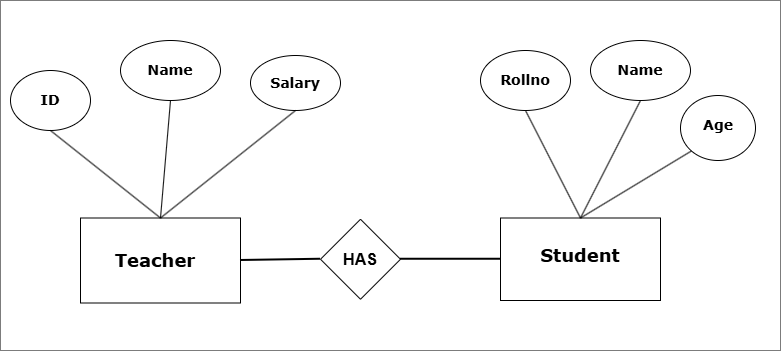
The above E-R model shows a conceptual school database with two entity sets – Teacher and Student.
The data is stored as tables with rows and columns in the database.
For example,
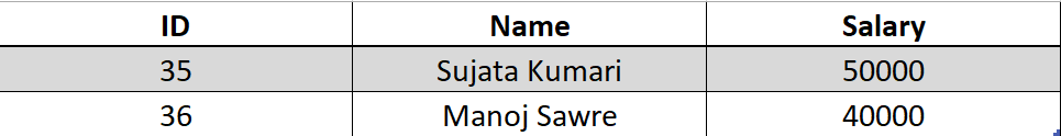
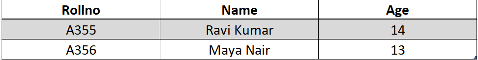
Relationships in Relational Model
Compared to hierarchical model and the network model, the relational model is more flexible. Yet, it employs data abstraction at all levels and provide data integrity and security.
The relationships in relational model is supported by cardinality ( number of entities in the relation). It supports following models:
- One-to-One (1:1)
- One-to-Many (1:N)
- Many-to-One (N:1)
- Many-to-Many (N:M)
Advantages of Relational Model
The relational model has many advantages.
- Simplicity – It is simple to use. The storage is in the form of table with rows and columns.
- Data Integrity – Each table has constraints such primary keys, and rules for attributes which maintain high accuracy in storing data.
- Data independence – Each level of this model is independent of high levels.
- Transactions are ACID compliant – Each transaction either complete successfully or fail and do nothing. The follow ACID properties – Atomicity, Consistency, Isolation, and Durability.
- Flexibility – Unlike Hierarchical model, or Network model, we can easily update tables and records.
- SQL – Relational model provides special query language to retrieve information from the database.
In future posts, you will only learn about Relational data model.
Summary
Data model is about how data is structured, organized, and represented in database systems. There are three levels of data model.
- Conceptual
- Logical
- Physical
There are different types of logical models in database system. The three main types are:
- Hierarchical model – Stores data as a tree based structure.
- Network model – stores data as a graph-like structure.
- Relational model – stores data in tables with rows and columns.
Program to Implement Kaprekar Routine for n-Digit Numbers
The program to implement Kaprekar Routine for n-digit numbers is based on Indian Mathematician D.R. Kaprekar constant \Large 6174 . The Kaprekar routine always converge to this constant – \Large 6174 for any \Large n digit number.
Rules for Input Numbers for Kaprekar Routine
The basic rules to chose a number for Kaprekar routine is:
- Number must be a 4-digit number. The fall in the range \Large 1 \leq n \leq 9999.
- If the number is smaller number, \Large 0 ‘s used to show the number as a 4-digit number. for example, \Large 23 is represented as \Large 0023.
- Repetition allowed but, only \Large 3 digits out of \Large 4 are repeated. For example, \Large 1222 is a valid number, but ,\Large 3333 is invalid.
The Kaprekar Routine
Once you selected a four digit number. We can apply the Kaprekar routine to it and get the end result in less than or equal to 7 steps. The final result of the routine is \Large 6174.
Step 1: Choose a number
Suppose we choose any arbitrary number such as \Large 3968.
The number is 4-digit number and it has at no repeating digits.
Step 2: Arrange digits of the number in descending order
Next, we must arrange the digits in descending order to get the largest possible number from the digits.
\Large 3968 \rightarrow 9863
After sorting the new number is \Large 9863.
Step 3: Arrange the digits of new number in ascending order
We must arrange the digits of new number from step 2 in ascending order ( smallest to largest ). In this way, we get the smallest possible number from the digits.
\Large 9863 \rightarrow 3689
The smallest number obtained from digits of \Large 9863 are \Large 3689.
The largest number obtained and smallest number from step 3 will be used to get the Kaprekar constant.
Step 4: Subtract the smallest number from the largest number
In this step, you need the largest number obtained in step 2 and the smallest number obtained from step 3. Subtract this two numbers to get a result.
 \Large \begin{aligned} & \hspace{16px} 9863 \\
&- 3689 \\
&\rule{2cm}{0.5px}\\
&\hspace{16px} 6174\\
&\rule{2cm}{0.5px}\\
\end{aligned}
Step 5: Repeat step 1 – 4 until you get the Kaprekar constant – 6174
The step 5 is about repeating the routine until you find the Kaprekar constant which is the number \Large 6174.
If you repeat the Kaprekar routine for any n-digit number repeatedly, the end result is \Large 6174.
The Kaprekar routing move from random number to structured difference of number (Largest – Smallest) and by repeating the subtraction procedure, you reach a stable number \Large 6174.
The result of Kaprekar routine on random number \Large 3968 is the stable constant \Large 6174.
Lets take another example, \Large 4386. The Kaprekar routine will produce following numbers.
\Large \begin{aligned}
8643 - 3486 = 5175\\
7551 - 1557 = 5994\\
9954 - 4599 = 5335\\
5533 - 3355 = 1998\\
9981 - 1899 = 8082\\
8820 - 0288 = 8532\\
8532 - 2358 = 6174
\end{aligned}
See the program for Kaprekar routine on a \Large 4386 below.
#include <stdio.h>

void sort(int a[])
{
    int i, j, temp;
    for (i = 0; i < 4; i++)
    {
        for (j = i + 1; j < 4; j++)
        {
            if (a[i] > a[j])
            {
                temp = a[i];
                a[i] = a[j];
                a[j] = temp;
            }
        }
    }
}

int main()
{
    int num, a[4], b[4], c[4], i;
    int count = 0;

    printf("Enter a 4-digit number: ");
    scanf("%d", &num);

    while (num != 6174)
    {
        // split digits
        a[0] = num / 1000;
        a[1] = (num / 100) % 10;
        a[2] = (num / 10) % 10;
        a[3] = num % 10;

        // sort ascending
        sort(a);

        // copy ascending to b
        for (i = 0; i < 4; i++)
            b[i] = a[i];

        // reverse a to make descending
        for (i = 0; i < 2; i++)
        {
            int temp = a[i];
            a[i] = a[3 - i];
            a[3 - i] = temp;
        }

        // subtraction: descending - ascending
        for (i = 3; i >= 0; i--)
        {
            if (a[i] < b[i])
            {
                a[i - 1]--;
                a[i] += 10;
            }
            c[i] = a[i] - b[i];
        }

        // convert array to number
        num = c[0] * 1000 + c[1] * 100 + c[2] * 10 + c[3];

        count++; // increment iteration count

        printf("Step %d: %d\n", count, num);

        if (num == 0) break; // safety check
    }

    printf("\nTotal iterations = %d\n", count);

    return 0;
}
#include <iostream>
#include <algorithm>
using namespace std;
void sortAsc(int a[])
{
sort(a, a + 4);
}
int main()
{
int num;
int a[4], b[4], c[4];
int count = 0;
cout << "Enter a 4-digit number: ";
cin >> num;
while (num != 6174)
{
// split digits
a[0] = num / 1000;
a[1] = (num / 100) % 10;
a[2] = (num / 10) % 10;
a[3] = num % 10;
// sort ascending
sortAsc(a);
// copy ascending to b
for (int i = 0; i < 4; i++)
b[i] = a[i];
// reverse to descending
reverse(a, a + 4);
// subtraction: descending - ascending
for (int i = 3; i >= 0; i--)
{
if (a[i] < b[i])
{
a[i - 1]--;
a[i] += 10;
}
c[i] = a[i] - b[i];
}
// convert to number
num = c[0] * 1000 + c[1] * 100 + c[2] * 10 + c[3];
count++;
cout << "Step " << count << ": " << num << endl;
if (num == 0)
break;
}
cout << "\nTotal iterations = " << count << endl;
return 0;
}import java.util.Arrays;
import java.util.Scanner;
public class Kaprekar {
static void sortAsc(int[] a) {
Arrays.sort(a);
}
public static void main(String[] args) {
Scanner sc = new Scanner(System.in);
int num;
int[] a = new int[4];
int[] b = new int[4];
int[] c = new int[4];
int count = 0;
System.out.print("Enter a 4-digit number: ");
num = sc.nextInt();
while (num != 6174) {
// split digits
a[0] = num / 1000;
a[1] = (num / 100) % 10;
a[2] = (num / 10) % 10;
a[3] = num % 10;
// sort ascending
sortAsc(a);
// copy ascending to b
for (int i = 0; i < 4; i++)
b[i] = a[i];
// reverse to descending
for (int i = 0; i < 2; i++) {
int temp = a[i];
a[i] = a[3 - i];
a[3 - i] = temp;
}
// subtraction: descending - ascending
for (int i = 3; i >= 0; i--) {
if (a[i] < b[i]) {
a[i - 1]--;
a[i] += 10;
}
c[i] = a[i] - b[i];
}
// convert array to number
num = c[0] * 1000 + c[1] * 100 + c[2] * 10 + c[3];
count++;
System.out.println("Step " + count + ": " + num);
if (num == 0)
break;
}
System.out.println("\nTotal iterations = " + count);
sc.close();
}
}def kaprekar(num):
count = 0
while num != 6174 and num != 0:
digits = list(f"{num:04d}") # ensure 4 digits with leading zeros
asc = int("".join(sorted(digits)))
desc = int("".join(sorted(digits, reverse=True)))
num = desc - asc
count += 1
print(f"Step {count}: {num}")
print("\nTotal iterations =", count)
num = int(input("Enter a 4-digit number: "))
kaprekar(num)The goal of the program is count the number of iterations to reach Kaprekar constant for any number. The program has following functions:
- Arrange the given number in largest using its digits.
- Get the a smallest number by reversing the largest number obtained in step1.
- Subtract the smallest number from largest to get results.
- Check if the result = \Large 6174.
- If not repeat step 1 to 4.
- If yes, exit the program and display number of steps to reach Kaprekar constant.
Output of the Program
Enter a 4-digit number: 4386
Step 1:  5175
Step 2:  5994
Step 3:  5355
Step 4:  1998
Step 5:  8082
Step 6:  8532
Step 7:  6174

Total iterations = 7File Handling Programming Examples
This page contains all file handling programming examples.
Learn to code in four different programming languages – C, C++, Java, and Python.
Structure/Class-based Programming Examples
This page contains all structure/class-based programming examples. Learn programming with our easy to understand examples in C, C++, Java, and Python programming languages.
Function-Based Programming Examples
This page contains all function-based programming examples.
Learn to code with four different languages – C, C++, Java, and Python with our easy to understand example programs.
String Programming Examples
This page contains all string programming examples. Learn to code in four different programming languages – C, C++, Java, and Python.
Array Programming Examples
This page contains all array programming examples. Learn program coding in four different languages – C, C++, Java, and Python.
Loop and Pattern Programming Examples
This page contains all loop and pattern programming example programs.
Mathematical Programming Examples
This page contains mathematical programming examples.