OS Swapping Processes
We have an intuitive understanding of process and process states from an earlier post now. If you want to know about process states and state transitions see link below.
Process States in Operating System
One of the states is the waiting state in which the process is waiting for some event or an I/O operation to complete. However, if too many processes are waiting, then the memory becomes full and there is no space for a running process.
The waiting processes are swapped out and swapped in, to free more memory for running processes.
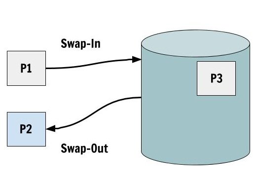
Swap-In and Swap-Out
This is a very simple technique in which a process get Swapped-Out of the memory to the disk because it will not be used for some time and whenever the process is required, it is Swapped-In from the disk.
Suspended States
The waiting states are also called the Blocked states. This block state becomes suspended state after it is swapped out to the disk. We now get to new suspend states
- Blocked-Suspend State
- Ready-Suspend State
In the Block-Suspend state, the process cannot do anything because it is swapped-out and blocked. The Ready-Suspend state is a state in which the process is swapped out and waiting for some event to happen so that it can become ready again.
The external storage used for Swapping-In and Swapping-Out of processes is called Page File.
Updated Process State Diagram
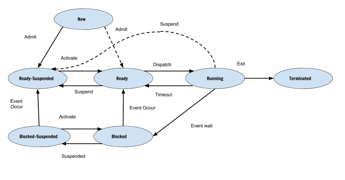
Transition Between States
There are no new states, therefore the transition of states include these new states.The list of new transition is as follows
- Block State – Block Suspended
- Block Suspended – Ready Suspended
- Ready – Ready Suspended (when some higher priority process comes)
- Block Suspended – Block When there is process with higher priority than ready)
- New – Ready Suspended
Summary
The process Blocked and then swapped out to free some memory when the process is not likely to be used for some time. This lead to two new process states – Block Suspended and Ready Suspended
References
- Abraham Silberschatz, Peter B. Galvin, Greg Gagne (July 29, 2008) Operating System Concepts, 8 edn., : Wiley.
- Ramez Elmasri, A Carrick, David Levine (February 11, 2009) Operating Systems: A Spiral Approach, 1st edn., : McGraw-Hill Education.
- Tanenbaum, Andrew S. (March 3, 2001) Modern Operating Systems, 2nd edn., : Prentice Hall.
OS Process States
When a computer program runs but only a part of a program is running performing a specific task. This smallest unit of a program in execution is called a process. Technically, a process is not the smallest unit but some programs consist of threads which are smaller than a process.
When there is no process then the state is null. However, when a process is created then it changes many states during its lifetime. The state information for a process is kept in a Process Control Block (PCB).
Process States
- New State – The process is created recently.
- Running State – The process is being executed currently.
- Waiting State – Waiting for some Event or Input/Output to finish, etc.
- Ready State – Just before being assigned to a processor.
- Terminated – The process finished execution.
Process State Diagram
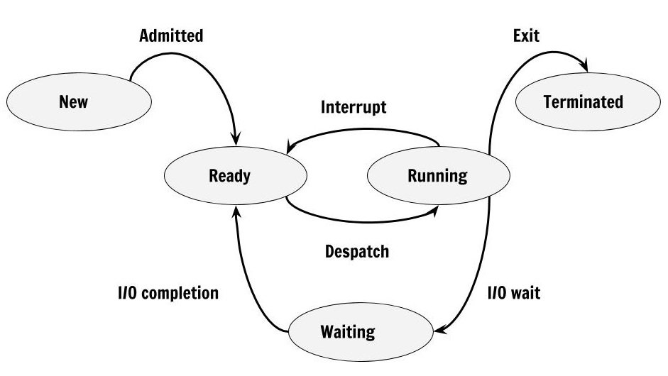
The figure above shows that process change states due to various reasons and here is a list of transitions that happen between processes. Not necessarily in the same order.
- Null -> New
- New -> Ready
- Ready -> Running
- Running -> Terminated
- Running -> Blocked
- Blocked -> Ready
- Running -> Ready
- Ready -> Terminated
- Waiting -> Terminated
Note – Running – Ready (This happens when process is removed from running due to a scheduling algorithm such as Round Robin, Priority Queue).
Summary
Process is program in execution and does specific task. The process changes may states during it’s life time and the final state for a process is Terminated state when it exits and no longer available in memory.
References
- Abraham Silberschatz, Peter B. Galvin, Greg Gagne (July 29, 2008) Operating System Concepts, 8 edn., : Wiley.
- Tanenbaum, Andrew S. (March 3, 2001) Modern Operating Systems, 2nd edn., : Prentice Hall.
SJF Tabular Method
In the previous article, we computed the average waiting time and average turnaround time for processes that are scheduled with First Come, First Serve (FCFS) algorithm using Tabular Method.
Introduction
In this post, we will compute average waiting time and average turnaround time for scheduled processes with another algorithm called Shortest Job First (SJF). You may have already seen an example of SJF in the previous post when we changed the order of the process in FCFS. In shortest job first algorithm, the process with shortest burst time is scheduled first for CPU time.
There is two version of this algorithm.
1. Preemptive.
2. Non-Preemptive
The preemptive version is also known as Shortest-Job-Remaining-Time and Shortest-Job-First is the non-preemptive version. For example, consider following scheduled processes.
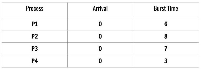
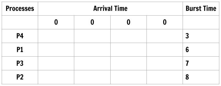
We see that there are 4 processes scheduled according to Shortest-Job-First and the arrival time of the processes is the same which is 0.
The burst time decides the order of the processes for CPU scheduling. The order is a job with lowest burst time has the highest priority.
P4 -> P1 -> P3 -> P2We will use this order in Tabulation Method for computing average wait time and turnaround time as follows.
The table has process ordered according to shortest job first algorithm and the arrival time is the same for each process. The order of the process is most important for this method to work and the order is decided by the burst time for each process.
Let’s fill the table according to burst time of each process in such a way that only upper triangular part has the entries and lower triangular part of arrival time is not filled. Also, each row next to the process will have only burst time of that process and nothing else.

Each column total is nothing but Turnaround time for the process. Therefore,
\begin{aligned}
&Average \hspace{3px} Turnaround \hspace{3px} Time = \frac{(3 + 9 + 16 + 24)}{4} = \frac{52}{4} = 13 \hspace{3px}ms
\end{aligned}
The first process in the order is P4 whose wait time is 0 and the first three column total gives wait time for the process – P1, P3, P2 respectively.
\begin{aligned}
&Average \hspace{3px} Waiting \hspace{3px}Time = \frac{0 + 3 + 9 + 16)}{4} = \frac{28}{4} = 7 \hspace{3px} ms
\end{aligned}
Shortest Job First (SJF) with Different Arrival Time
Shortest Job First Scheduling with a different arrival time for each process add more complexity, but you will find it easy with the Tabular Method. You can easily compute the average waiting time and average turnaround time.
However, you have to consider these very important points before drawing a table.
- First, consider the arrival time of the processes.
- Next, select the process with the smallest burst during that arrival time.
- Reiterate the first and the second step for next arrival time.
- Order the arrival times according to the order of processes.
Consider another schedule of processes,
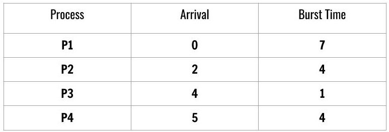
At this time, the processes are not ordered according to SJF and arrival time is not ordered. We order the process and the arrival time for Tabulation method.

To compute individual turnaround time of each process we subtract the total of each column with arrival time. The processes are ordered as follows
\begin{aligned}
&Process \hspace{3px}Order: \hspace{2em}P1 \rightarrow P3\rightarrow  P2 \rightarrow P4\\\\
&Arrival \hspace{3px}time \hspace{3px}Order:0 \hspace{2.5em}4  \hspace{2.2em} 2    \hspace{2.5em}    5\\\\
&Average \hspace{3px}Turnaround \hspace{3px}Time = \frac{(7 + 4 + 10 + 11)}{4 }= \frac{32}{4 }= 8 \hspace{3px}ms\\\\
&Waiting\hspace{3px} time = (Column\hspace{3px} Total \hspace{3px}of \hspace{3px}current \hspace{3px}process - Burst \hspace{3px}time \\
&of \hspace{3px} the \hspace{3px}process)
\end{aligned}
To compute the waiting time of each process using the following formula.
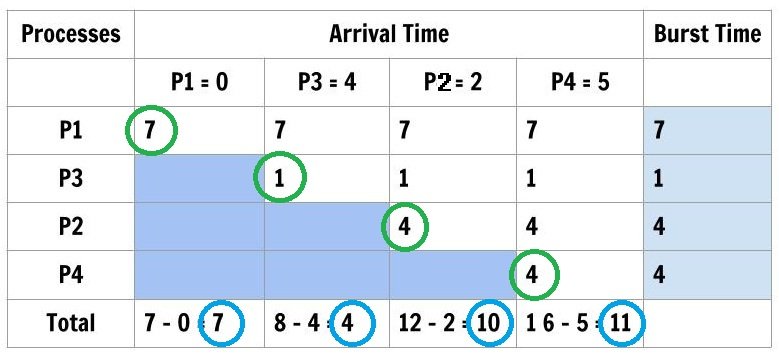
Waiting Time of each process
\begin{aligned}
&P1 = 7 - 7 = 0\\
&P3 = 4 - 1 = 3\\
&P2 = 10 - 4 = 6\\
&P4 = 11 - 4 = 7\\
&Average \hspace{3px} Waiting \hspace{3px} Time = \frac{(0 + 3 + 6 + 7)}{4} = \frac{16}{4} = 4 \hspace{3px}ms
\end{aligned}
Conclusion
The computation with different arrival time is difficult but systematic with Tabular Method, instead of using a Gantt Chart. There will be no mistakes in computation. In the next post, we will use Tabular Method to compute the CPU Scheduling times for Priority Scheduling.
References
- Abraham Silberschatz, Peter B. Galvin, Greg Gagne, A Silberschatz. 2012. Operating System Concepts, 9th Edition. Wiley.
FCFS Tabular Method
The usual method of computing average time, average wait time, turnaround time and average turnaround time for processes is to make a Gantt Chart and then compute these times. In this article, we explore another way to compute the average turnaround time and average wait time for processes based on the same logic given by the specific algorithm.
CPU Scheduling Algorithms
In the previous article, you learnt how tabular method computer the turnaround time and wait time for SJF algorithm. The popular CPU scheduling algorithms are as follows
- First Come, First Serve
- Shortest Job First
- Priority Scheduling
- Round Robin
This article, we use tabular method on FCFS (first come, first serve). Throughout the post, we will use the same example to compute the times using FCFS. Consider the following processes.
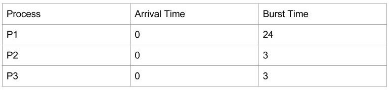
We will compute the average turnaround time and average wait time for the processes using the tabular method.
First Come, First Serve
At first, make a table as follows, with processes ordered in the way they arrive in the queue.
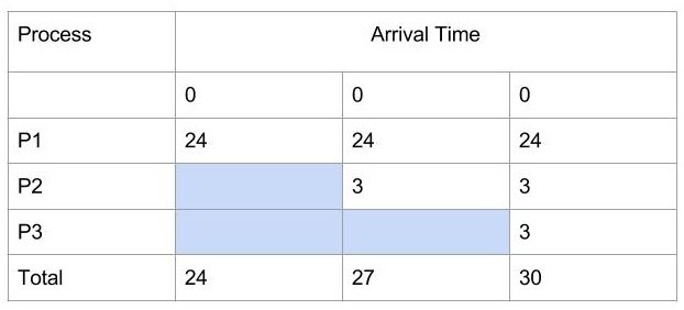
The first column is for processes in the ready queue and listed in the order as they arrive. The arrival of all three processes is 0.
- Fill the first row with burst time of process P1.
- Fill the second row with burst time of process P2 because it starts after P1.
- Similarly, fill the burst time of P3 in the third row last column because P3 start after P2 process.
- Each column is Turnaround time for each process in the queue.
\begin{aligned}
&Average \hspace{3px}Turnaround \hspace{3px} Time = \frac{(24 + 27 + 30)}{3 }= \frac{81}{3} = 27 \hspace{3px} ms
\end{aligned}
Note: waiting time of the first process is always 0.
To compute the average waiting time of each process, add all the value in row Total, except the last column and divide by a number of processes.
\begin{aligned}
&Average \hspace{3px}Waiting \hspace{3px}Time = \frac{(0 + 24 + 27)}{3 }= \frac{51}{3} = 17 \hspace{3px}ms
\end{aligned}
First Come, First Serve with Change in Order
Suppose we change the order of execution. Does that change the average waiting time and turnaround time of the processes scheduled using the FCFS, let’s find out the answer.
\begin{aligned}
&Average \hspace{3px}Turnaround \hspace{3px}Time = \frac{(3 + 6 + 30)}{ 3 }= 13 \hspace{3px}ms \\\\
&Average \hspace{3px}Waiting \hspace{3px}Time = \frac{(0 + 3 + 6)}{3 }= 3 \hspace{3px}ms
\end{aligned}
In the above example, process P3 is the first, process P2 is second and process P4 is the third in that order. We already know the wait time of the process P3 = 0 because it is the first process to arrive in the queue.
For turnaround time take the total of row “Total” and divide by 3 will give you the answer and for the average waiting time, the sum of first two columns of the row “Total” divided by 3 will give you the answer.
First Come, First Serve with different Arrival Times
Consider another example, here process arrive at the ready queue with different times.
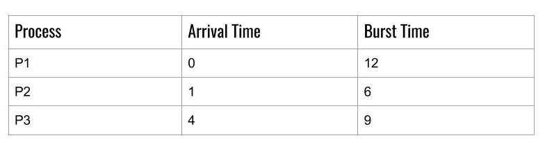
To compute the average turnaround time and average waiting time using the tabular method. Draw following table but this time we have different arrival times for each process.
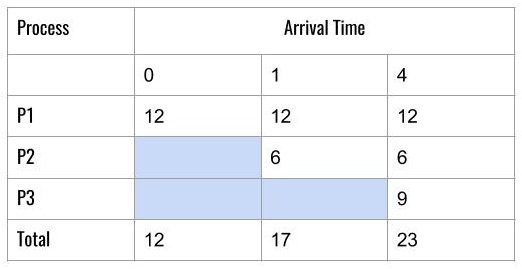
To calculate the individual Turnaround time for each process, we need to take the column total for minus the arrival time in the same column.
For example
\begin{aligned}
&In \hspace{3px}the  \hspace{3px}first \hspace{3px}column,\\&we  \hspace{3px}have  \hspace{3px}a  \hspace{3px}Total = 12 - 0  \hspace{3px}(Arrival  \hspace{3px}Time) \\&= 12 \hspace{3px}( Turnaround  \hspace{3px}time  \hspace{3px}for  \hspace{3px}P1)\\\\
&In  \hspace{3px}the  \hspace{3px}second  \hspace{3px}column, \\&we \hspace{3px} have  \hspace{3px}a  \hspace{3px}Total = 18 - 1( Arrival  \hspace{3px})\\& = 17 ( Turnaround  \hspace{3px}time  \hspace{3px}for P2)\\\\
&Average  \hspace{3px}Turnaround  \hspace{3px}time = \frac{(12 + 17 + 23)}{3} = \frac{52}{3} = 17.33  \hspace{3px}ms.
\end{aligned}
To compute the waiting time of each process, take each column total – next process arrival time and you get the results.
For example
\begin{aligned}
&waiting \hspace{3px}time \hspace{3px}for \hspace{3px}P1 = 0\\\\
&waiting \hspace{3px}time\hspace{3px} for\hspace{3px} P2 = 12 - 1 = 11\\\\
&time \hspace{3px}for \hspace{3px}P3 = 18 - 4 = 14\\\\
&Average \hspace{3px}Waiting \hspace{3px}Time = \frac{(0 + 11 + 14)}{3} = \frac{25}{3} = 8.33 \hspace{3px}ms
\end{aligned}
Conclusion
The tabular method employs the same method as performing calculations using Gantt Char but if the number of processes and other data becomes too complex then you may tend to make mistakes. Then using the Tabular method simplifies the calculations.
In the next post in this series, we will see more complex examples and how they can be tackled using this method of calculation.
References
- Abraham Silberschatz, Peter B. Galvin, Greg Gagne, A Silberschatz. 2012. Operating System Concepts, 9th Edition. Wiley.
Page Table
Most OS allocate a page table for each process. A pointer to the page table is stored in the PCB of the process. When the dispatcher start a process, it must reload the user registers and define the correct hardware page table from the stored user page-table.
Hardware Page Table
The hardware page table can be implemented in many ways. The simplest form of page table can be build using high speed registers for better efficiency. The CPU dispatcher reloads these register-like other registers and instructions to modify the page-table registers are privileged, so only OS can change the memory map.
Example, DEC PDP-11
The address has 16-bit and page-size is 8 KB.
The use of registers is good for memory with small size such as 256 entries in page table. But, in modern computer the size of entries is 1 million cannot use fast registers.
Memory Page Tables
The page-table is kept in main memory and a page-table base register (PTBR) points to the page table. To change page-table entries, you only need to change the value of PTBR.
To access memory location i, we must index into the page-table, using the value in the PTBR, offset by page number for i. This provides us with a frame number and together with offset value gives us the physical address. Then we can access the memory.
This scheme requires two memory access for a byte, therefore, slowed the memory access by a factor of 2.
1. One memory access for the page-table entry
2. Another memory access for the byte.
The above approach is also slow.
The standard solution is to use a Translation Look-aside Buffer (TLB).
- The TLB is associative, high-speed memory.
- Each entry consist of two parts – a key or a tag and a value.
- When an item is presented, it is compared with all the keys. If a match is found, then the corresponding value is returned.
- Number of entries in TLB is small, usually between 64-1024.
TLB With Memory Page Table
The working of TLB is as follows:
- CPU generates the logical address.
- Its page number is presented to TLB.
- If page is found, obtain frame number
- Access the memory.
- If not page not found, it is called TLB miss, a memory reference to the page table must be made.
- When frame number obtained, use it to access memory.
- Add the page and frame number to the TLB, so next reference we can find it quickly.
- If the TLB is full, then OS must use one entry for replacement (using page replacement algorithm).
Other Features Of TLB
- Some entries are wired down(cannot be replaced). The TLB entries for kernel code are wired down.
- Some TLB store address-space identifiers (ASIDs) in each TLB entry. An ASID uniquely identify process and provide address space protection for that process.
- TLB tries to resolve a virtual page, if ASID of process and a virtual page does not match. It is a TLB miss.
- For several processes, if TLB does not support separate ASIDs, then flush or erase TLB for next executing process.
- Otherwise, TLB will refer to valid virtual addresses of previous process and refer to incorrect physical addresses.
The percentage of time a page is found in the TLB is called a hit ratio.
An 80% hit ratio means pages are found 80% of time. If it takes 20 nanoseconds to search TLB. If it takes 100 nanoseconds to access memory.
then,
It takes 120 nanoseconds for mapped-memory access when page is in TLB.
If the page is not found in TLB which takes 20 nanoseconds
It takes 100 nanoseconds to access the page-table in memory.
It takes 100 nanoseconds to access the byte from memory.
The total of 220 nanoseconds to access memory.
To find the effective memory access time, we weight the case by its probability:
\begin{aligned}
&Effective  \hspace{3px}memory  \hspace{3px}access  \hspace{3px}time = 80/100 * 120 + 20/100 * 220\\\\
&= 96 + 44 = 140  \hspace{3px}nanoseconds.
\end{aligned}
The slowdown is 40% (from 100 to 140 nanoseconds)
For 98% hit ratio,
\begin{aligned}&Effective \hspace{3px} access \hspace{3px} time = 98/100 * 120 + 2/100 * 220 \\\\&= 196 117.6 + 4.4 = 122 nanoseconds\end{aligned}The increased hit ratio produces only 22 % slowdown.
Memory Protection in Paging
Memory protection in paged environment is accomplished by protection bit with each frame number. These bits are kept in the page-table. One bit can define page to be read-write or read-only.
When the page physical address is being computed, the protection bit is verified to prevent write on a read-only page. If such an attempt is made then it cause a hardware trap.
One additional bit is included with each entry, a valid-invalid bit by operating system. If the bit is set to valid, the page is in the process’s virtual address space. If bit is set to invalid, the page is not in virtual address space, resulting in a trap.
Suppose a 14-bit address space, with page size  . The number of pages is
14 - 11 = 3 = \frac{2^{14}}{ 2^{11}}= 2^3= 8 \hspace{3px} pagesIf the process is restricted to use only 0 to 10453, then all other addresses are set to invalid. The invalid address inside a page are unused and cause internal fragmentation.
 page (10240 addresses) + 213 addresses. But the entire 6th page is considered as valid. This is internal fragmentation.
Memory Mapping Schemes
Memory mapping is a technique to bind user-generated addresses to physical addresses in the memory. This requires static binding or dynamic binding.
CPU gets instruction from memory, and then decode the instruction during the instruction-execution cycle. The instruction also contains the memory address of operands that need to be fetched. The CPU finished the instruction and saves the results back to memory. The memory unit only sees streams of addresses and does not know how they are generated.
Memory Hardware
A CPU can only access registers and memory directly. The processes that are on disk must be brought to memory before CPU operates on them.
There is two concern for the CPU:
- The speed of access to memory.
- The memory protection.
The CPU is fast compared to memory, if the data is not available to CPU, it tries to access the memory or it will remain idle or stop working. To increase the speed of access a fast memory called cache is included in the system which stores frequently used data.
The memory protection is implemented by CPU using two registers – base and limit. The base contains the lowest physical address and limit contains the range of address.
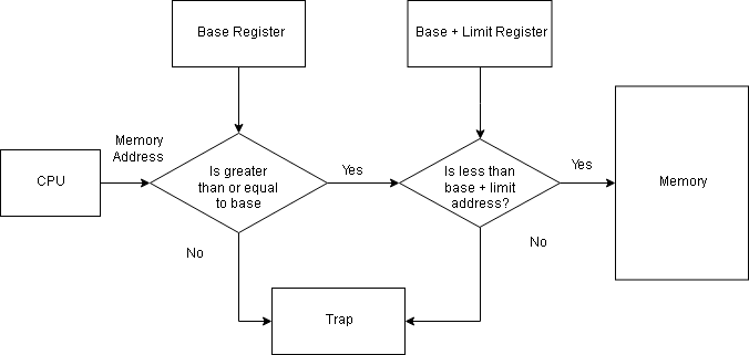
Each user-generated address is compared with the base and limit to determine the legitimacy of the address. A trap is generated if the user process tries to access OS memory. The OS runs in privileged mode or kernel mode and has full access to all the memory.
Memory Mapping Techniques
A program is bought to memory as process and keeps moving between disk and memory, depending on the memory management. All processes waiting to be loaded into memory form an input queue.
Normally, one process is selected from the queue and it is executed in memory. When the process terminates, its memory is free.
The system allows the user process to reside in any part of the physical memory. The memory starts at 00000, but the user process starting address need not be 00000.
The user process goes through several mapping steps before it gets executed:
- The address at source code is symbolic addresses. E.g total = 23;.
- The compiler binds the symbolic address to relocatable addresses ( e.g 10 bytes from the beginning of this module).
- The linkage editor or loader will in turn bind the relocatable address to absolute address such as 43267.
The binding is a mapping of one address to another which can be done in many ways;
Compile time mapping
If you already know that a process will start at memory location M, then compiler code will start at that location and generate absolute code directly. The code and data references are mapped to physical addresses when program is compiled. If the location changes then, recompile the code.
E.g MS-DOS.COM-format programs are bound at compile time.
Load time mapping
If the memory location of the process is not known, the compiler must generate relocatable code. This binding process adds a starting address of the process to each reference in the program. The process will not move to another memory location during execution because starting address must remain the same. If starting address changes, reload the user code to incorporate the change. The final binding is delayed until load time.
Execution time mapping
In this method, a virtual address is mapped to a physical address. If the process can be moved from one memory location to another, then binding is delayed until runtime. It requires special hardware and most OS use this method.
References
- Linda Null, Julia Lobur (December 17, 2010) The Essentials of Computer Organization and Architecture, 3rd edn., Jones & Bartlett Learning.
- Abraham Silberschatz, Peter B. Galvin, Greg Gagne (July 29, 2008) Operating System Concepts, 8 edition edn., Wiley.
Logical Directory Structures
The directory have a logical structure that defines how files are organized inside the directory. There are many organizing schemes such as single level, two level, tree structure, and acyclic-graph structure. In this article, you will learn about various logical directory structures and need for them.
Single Level Directory
It is the simplest directory structure with all files in the same directory which easy to access, support and understand.
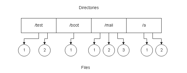
Disadvantages
Few disadvantages with a single level directory are:
- When files increase, they are very difficult to manage.
- The files must have unique names because multiple users can have same filenames.
- A user may not remember the filenames because of too many files in the same directory.
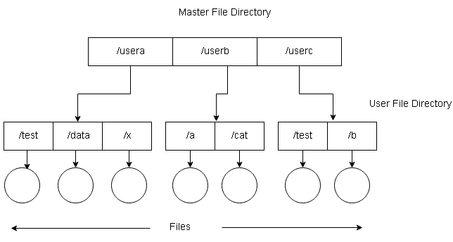
Two level directories
In single level directory, it is difficult to manage each user files. The two level directory system allows a directory
called User File Directory(UFD) which only list files of a single user.
When user logs or starts a job, a Master File Directory (MFD) is searched for a user name or account number. The MFD is indexed on user name or account number and each entry points to a UFD.
When user searches for a file he refers to his own UFD. A file name is unique within the UFD even with the same
name by different users.
User can create files, delete files, rename files, and so on by searching for an existing file before performing a file
operation. Administrators can delete the UFD and create a new one and adds an entry into the MFD.
Disadvantages of Two-Level Directory
We list here the disadvantages of a two-level directory structure.
- Isolates one user from another which is a problem if the system needs cooperation between users on certain projects or tasks.
- One user cannot access files of other users unless permission is given explicitly.
Directory Path
The MFD and UFD can be thought of as a tree where files are leaves of the tree. The UFD itself is a file in the tree and
make a path with a file name.
For Example:
A file name “test” in user B directory has path \userb\test\.
In MS-DOS, a volume is specified as a letter followed by a colon, C:\userb\test.
In VMS, u:[sst.jdeck]login.com;1 where u: is volume, sst is a directory, jdeck is subdirectory and login.com is file
name.
Some other systems treat volume as directory, /u/pub/test where u is a volume.
The system files are part of a loader, compilers, utility routines, libraries, and assemblers. The operating system receives commands with filenames, the command line interpreter search for requested filenames in UFD, then load and execute the files.
This means that we need to keep a copy of system files for each user. If system files are 5 Mb in size, then the total space required for 12 users would be 12 * 5 = 60 MB. This would be a waste of space to keep multiple copies of the same files.
The standard solution would be to create a special directory for system files. If search could not find any system files
in the local UFD, then search in the special directory.
A sequence of directories are searched when a file is named is called search path. This search path can be extended with unlimited directories to search. This a popular method of search in MS-DOS and UNIX.
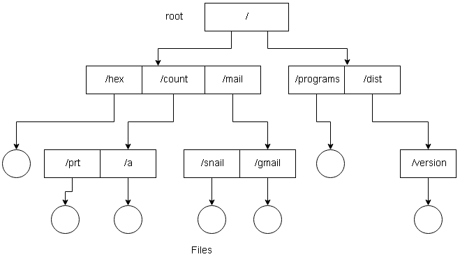
Tree-Structured Directory
The two-level directory structure could be extended to create a tree-structure with arbitrary height. The user can create subdirectories and keep their files.
The tree has a root directory and every file in the tree has a unique path name. A directory (or subdirectory) contains list of files or subdirectories. A single bit in each directory entry defines the content as file(0) or subdirectory(1).
Each process has a current directory which contains files that the process is currently interested in. If a referenced file is not in the current directory, the user must specify the path or change the current directory to be the directory holding the file.
Now, the user can change the directory using change directory system calls to another directory. The search path does not include an entry that stands for “the current directory”.
An initial current directory is assigned to the user when a job starts or when the user logs in. The accounting file contains entry to this initial current directory, therefore, a pointer for the operating system for the initial current directory. The current directory of any subprocess is the current directory of the parent.
The path name are of two types – absolute path and relative path in the tree structure.
- Absolute path – It is path to a file from the root directory given names of all directories and subdirectories in the path.
- Relative path – It is path from the current directory to the file including names of all directories and subdirectories in the path.
Deleting directories
There are two approaches to deleting directories and files from a tree-structure. The first approach used in MS-DOS, a directory cannot be deleted unless it has no files, and this applied to subdirectory as well.
The second approach used in UNIX operating system, using rm command you can delete a directory along with subdirectories and files. All with a single command. This option is dangerous if you do not have a backup of files to restore it later.
Tree structure directory allows users to access other user’s files and directories. They can do that by specifying absolute path or relative path to the file.
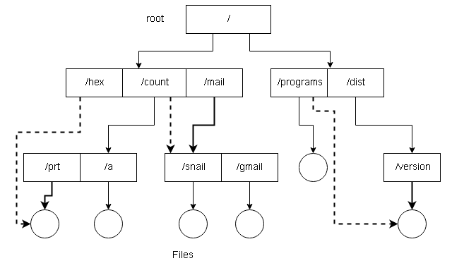
Acyclic-Graph Directories
A tree-structure does not allow sharing of files. The acyclic-graph (graph with no cycle) directories allow common shared directories for two or more users.
The shared file or directory will appear in two different places at the same time, but they are not copies and changes are done to a single file. Usually, teamwork requires such shared directories and subdirectories. One new file from a person in a shared subdirectory is replicated in all shared subdirectories.
Implementing Shared Files and Sub-directories
In UNIX system, a new directory entry is created called link. A link is a pointer to another file or subdirectory and implemented as an absolute path or relative path to the file or subdirectory.
When a reference is made to the file, then we search the directory, but the file is marked as a link with a path name. The system will resolve the link pathname to get the real file. While traversing the tree, the link entries are ignored to preserve the acyclic-graph structure.
Another approach is to duplicate all information about files in both sharing directories. The problem with this approach is consistency when the files are modified.
Disadvantages
The acyclic-graph structure is flexible than tree structure but more complex. We have listed some disadvantage of
this structure below.
- A File have multiple absolute paths. Traversing the file structure will cause a problem with multiple entries to the same file.
- Once the original file is deleted its space is deallocated, but it can leave dangling pointers which are pointing to the deleted file. If we keep a list of associated links and when the count of references becomes 0, it is a lot easier to remove link rather than searching links and remove them.
- We can leave the link dangling, only an attempt to resolve them will result in error.
An acyclic-graph directory ensures that there are no cycles in the structure. We start with two level directories, then add more subdirectories and files resulting in a tree structure. However, the tree-structure is broken when links are
added and it becomes a simple graph directory structure.
An acyclic graph traverses the graph to determine that there is no reference to a file. We want to avoid searching the
acyclic directory again for shared files or subdirectories if an attempt to find the file failed. This is for performance
reasons.
What if we allow cycles (self-referencing) in the directory structure? The search would never end. The possible
solution might be to avoid searching shared directories. When the link count becomes 0, the file is deleted. But the when cycle exist the count never becomes 0 and the search algorithm will go to a never terminating loop.
The solution to this problem would be garbage collection, in which two passes is made:
- The first pass will mark everything that is accessible.
- The second pass will add the rest of the items including links to free space list.
It is effective, but a time-consuming effort. The best solution, therefore, is to avoid traversing links.
References
- Abraham Silberschatz, Peter B. Galvin, Greg Gagne (July 29, 2008) Operating System Concepts, 8 edn., Wiley.
- Ramez Elmasri, A Carrick, David Levine (February 11, 2009) Operating Systems: A Spiral Approach, 1st edn., McGraw-Hill Education.
- Tanenbaum, Andrew S. (March 3, 2001) Modern Operating Systems, 2nd edn., : Prentice Hall.
Storage Structure
Files are stored on random-access storage devices including hard disks, optical disks, and solid-state disks. The storage device can entirely be used as a file system or divided into many partitions. Each partition may or may not have a different file system.
Storage devices are collected into RAID sets, that provides high availability and fault tolerance in case a disk fails. The partitions can also be used to create RAID sets.
Swap Space
The partitions are known as slices or mini disks. Sometimes partitions are left without any file system on them for other purposes such as swap space. Every partition should have a file system installed and such a partition is called volume.
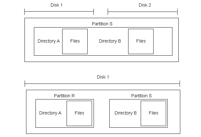
They are virtual disks that contain information about the file system in a device directory or volume table of contents. It contains information about name, size, location, and type of all the files in the volume. The volume can contain more than one operating systems that can run concurrently.
File System of Solaris
The computer system has storage devices that may have 0 or more file systems. Each file system may be different where some are general purpose and some special file systems. Here is a list of general-purpose file system used in Solaris.
tmpfs – temporary file system
objfs – virtual file which is interface to kernel that look like a file system and gives debuggers access to kernel
symbols.
ctfs – a virtual file system to maintain “contract” information to manage which process start when the system boots
and continue to run.
lofs – “loop back file system ” allows one file system to be accesses in place of another one.
procfs – a virtual file system that provide information on all processes as file system.
ufs, zfs – general-purpose file system
Directory Structure Overview
When we create a file within a directory and entry for the file is made to the directory. The directory can be
organized in may ways. Here is a list of operations performed on a directory.
Create a file – a new file is created and added to the directory.
Delete a file – an existing file and its entry is deleted from the directory.
List a directory – display the all files inside directory and directory entries for each of these files.
Rename a file – A user with proper permission can rename a file. It will change the position of the file in the
directory.
Traverse the file system – Certain situation demands to traverse the file system – visiting every directory and file in the file system such as taking a backup at regular interval. The backup copy of the file system is stored in a magnetic disk or hard drive.
References
- Abraham Silberschatz, Peter B. Galvin, Greg Gagne (July 29, 2008) Operating System Concepts, 8 edn., : Wiley.
File Access Methods
The information stored in a file must be accessed and read into memory. Though there are many ways to access a file, some system provides only one method, other systems provide many methods, out of which you must choose the right one for the application.
Sequential Access Method
In this method, the information in the file is processed in order, one record after another. For example, compiler and various editors access files in this manner.
The read-next – reads the next portion of a file and updates the file pointer which tracks the I/O location. Similarly, the write-next will write at the end of a file and advances the pointer to the new end of the file.
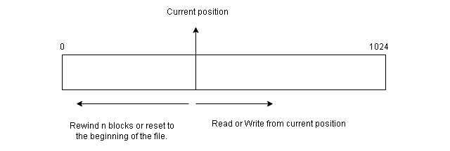
The sequential access always reset to the beginning of the file and then starts skipping forward or backward  records. It works for both sequential devices and random-access devices.
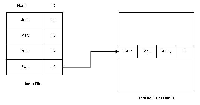
Direct Access Method
The other method for file access is direct access or relative access. For direct access, the file is viewed as a numbered sequence of blocks or records. This method is based on the disk model of file. Since disks allow random access to file block.
You can read block 34, then read 45, and write in block 78, there is no restriction on the order of access to the file.
The direct access method is used in database management. A query is satisfied immediately by accessing large amount of information stored in database files directly.
The database maintains an index of blocks which contains the block number. This block can be accessed directly, and information is retrieved.
The File Operations for Direct Access
Rather than read next or write next, the direct access method passes the block number as the parameter for read and write operations.
read n
write m
For example,
read 34
write 56
This is very similar to sequential access, but in addition to reading, the position the pointer to block 36 before a read or write operation.
The block number is a relative block number which is an index relative to the beginning of the file. Therefore, block 0 is the first relative block. The absolute disk location of the block may be 3553 and 4556 for the next block. This helps OS decide the placement of the file on the disk called the allocation problem.
If user requests for a record N and a record length is L, then the system should read or write from L * (N) within the file.
Not all systems provide sequential and direct access. They either provide sequential access or direct access. Some system request access method information when the file is created. The access to the file depends on the declarations on these types of systems.
References
- Abraham Silberschatz, Peter B. Galvin, Greg Gagne (July 29, 2008) Operating System Concepts, 8 edn., : Wiley.
File Type
The operating system should support the file system. If the OS does not recognize a file type then any operation on the file will not be successful. The files are given an extension to indicate the type of file separated by a period or a dot.
For example,
- finance.java – A java program source code file.
- program.c – A C program source code file.
- salary.doc – A MS Word document.
- flower.jpg – An image file.
The above are some examples of file types which information in the form of text, image, programming code, audio, video and binary files.
File Types in OS
The file type decide the operation on the file. You cannot read and image file, so you need an image viewer. Similarly, C source code file needs a C compiler, not any other programming language compiler.
Here is a list of common file types recognized by most operating systems.
| File Type | Extension | Description |
| executables | .exe, .com, .bin or none | machine language programs that can run immediately. |
| object | .o, .obj | compiled code that are not linked |
| source code | .c, .java, .cc, .asm, .a | source code in programming languages |
| batch | .bat, .sh | contains commands for command interpreter |
| text | .txt, .doc | text documents |
| word processor | .doc, .rtf, .rtf, .wp | word processor text documents |
| library | .lib, .a, .so, .dll | library of builtin functions |
| print or view | .jpg, .ps, .pdf | ASCII or binary files for printing or viewing |
| archive | .zip, .rar, .tar | related files grouped into one file |
| multimedia | .mpeg, .mov, .avi, .rm, .mp3 | binary files containing audio, video |
References
- Abraham Silberschatz, Peter B. Galvin, Greg Gagne (July 29, 2008) Operating System Concepts, 8 edn., : Wiley.