In the previous article, we computed the average waiting time and average turnaround time for processes that are scheduled with First Come, First Serve (FCFS) algorithm using Tabular Method.
Introduction
In this post, we will compute average waiting time and average turnaround time for scheduled processes with another algorithm called Shortest Job First (SJF). You may have already seen an example of SJF in the previous post when we changed the order of the process in FCFS. In shortest job first algorithm, the process with shortest burst time is scheduled first for CPU time.
There is two version of this algorithm.
1. Preemptive.
2. Non-Preemptive
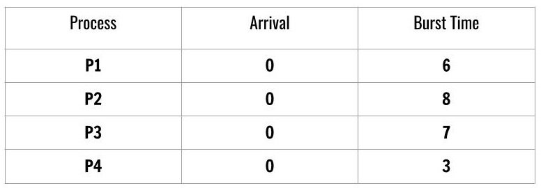
The preemptive version is also known as Shortest-Job-Remaining-Time and Shortest-Job-First is the non-preemptive version. For example, consider following scheduled processes.

We see that there are 4 processes scheduled according to Shortest-Job-First and the arrival time of the processes is the same which is 0.
The burst time decides the order of the processes for CPU scheduling. The order is a job with lowest burst time has the highest priority.
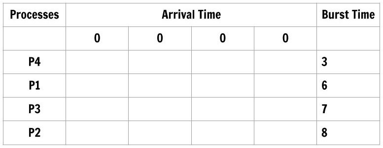
P4 -> P1 -> P3 -> P2We will use this order in Tabulation Method for computing average wait time and turnaround time as follows.
The table has process ordered according to shortest job first algorithm and the arrival time is the same for each process. The order of the process is most important for this method to work and the order is decided by the burst time for each process.

Let’s fill the table according to burst time of each process in such a way that only upper triangular part has the entries and lower triangular part of arrival time is not filled. Also, each row next to the process will have only burst time of that process and nothing else.

Each column total is nothing but Turnaround time for the process. Therefore,
\begin{aligned}
&Average \hspace{3px} Turnaround \hspace{3px} Time = \frac{(3 + 9 + 16 + 24)}{4} = \frac{52}{4} = 13 \hspace{3px}ms
\end{aligned}
The first process in the order is P4 whose wait time is 0 and the first three column total gives wait time for the process – P1, P3, P2 respectively.
\begin{aligned}
&Average \hspace{3px} Waiting \hspace{3px}Time = \frac{0 + 3 + 9 + 16)}{4} = \frac{28}{4} = 7 \hspace{3px} ms
\end{aligned}
Shortest Job First (SJF) with Different Arrival Time
Shortest Job First Scheduling with a different arrival time for each process add more complexity, but you will find it easy with the Tabular Method. You can easily compute the average waiting time and average turnaround time.
However, you have to consider these very important points before drawing a table.
- First, consider the arrival time of the processes.
- Next, select the process with the smallest burst during that arrival time.
- Reiterate the first and the second step for next arrival time.
- Order the arrival times according to the order of processes.
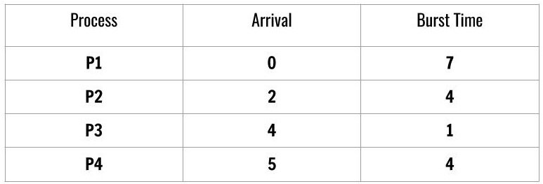
Consider another schedule of processes,

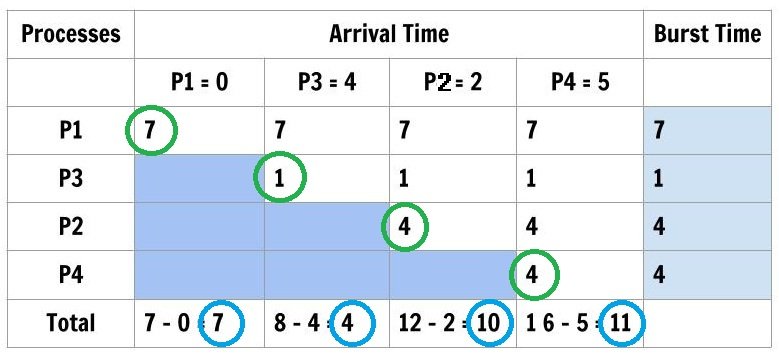
At this time, the processes are not ordered according to SJF and arrival time is not ordered. We order the process and the arrival time for Tabulation method.

To compute individual turnaround time of each process we subtract the total of each column with arrival time. The processes are ordered as follows
\begin{aligned}
&Process \hspace{3px}Order: \hspace{2em}P1 \rightarrow P3\rightarrow  P2 \rightarrow P4\\\\
&Arrival \hspace{3px}time \hspace{3px}Order:0 \hspace{2.5em}4  \hspace{2.2em} 2    \hspace{2.5em}    5\\\\
&Average \hspace{3px}Turnaround \hspace{3px}Time = \frac{(7 + 4 + 10 + 11)}{4 }= \frac{32}{4 }= 8 \hspace{3px}ms\\\\
&Waiting\hspace{3px} time = (Column\hspace{3px} Total \hspace{3px}of \hspace{3px}current \hspace{3px}process - Burst \hspace{3px}time \\
&of \hspace{3px} the \hspace{3px}process)
\end{aligned}
To compute the waiting time of each process using the following formula.

Waiting Time of each process
\begin{aligned}
&P1 = 7 - 7 = 0\\
&P3 = 4 - 1 = 3\\
&P2 = 10 - 4 = 6\\
&P4 = 11 - 4 = 7\\
&Average \hspace{3px} Waiting \hspace{3px} Time = \frac{(0 + 3 + 6 + 7)}{4} = \frac{16}{4} = 4 \hspace{3px}ms
\end{aligned}
Conclusion
The computation with different arrival time is difficult but systematic with Tabular Method, instead of using a Gantt Chart. There will be no mistakes in computation. In the next post, we will use Tabular Method to compute the CPU Scheduling times for Priority Scheduling.
References
- Abraham Silberschatz, Peter B. Galvin, Greg Gagne, A Silberschatz. 2012. Operating System Concepts, 9th Edition. Wiley.
