Integration Of Data Sources In Data Mining

After data cleaning steps in data mining. You need integration of data sources in data mining. It means combining disparate data sources into a single schematic structure.

There are two major type of integration – schema integration and data integration.

Schema integration forms an integrated schematic structure from the disparate data sources.

The data integration is about cleaning and merging data from different sources.

Schema Integration

Consider the following schemata:

Cars (serial No, model, color, stereo, glass-tint,...)
and
Auto(serienNr, modelle, farbe)

There are two tables and one in German. With this type of data there are few challenges listed below.

• Naming difference
• Structural difference
• Data type difference
• Missing fields
• Semantic differences

Generic Architecture of Integrator

The generic architecture of an integrator has components such as extractors, mediator, data sources.

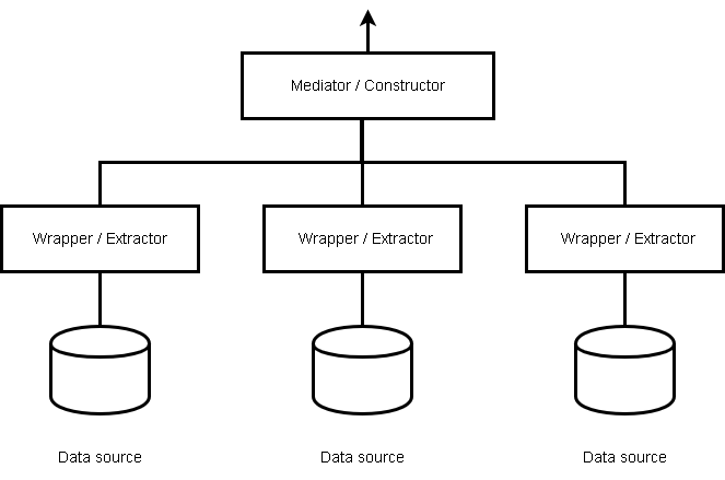
Extractor maps into a standard schema set. The extractors are responsible for transferring data from operational database to data warehouse.

Mediators constructs to overall schema. It is the one responsible for data integration from heterogeneous data sources.

Wrapper / Extractor

Creates a common view across all data sources. It bridges the differences in the naming, type and schema structure. Wrappers do not physically extract data from the data sources, but, send a local query to the target database. The result from this local query is converted into a relational form.

Mediator / Constructor

The mediator constructs an integrated schematic structure and performs data integration and populate the data warehouse.

Tools for Data Cleaning and Integration – dfPower

• It is from Dataflux corporation.
• has a de-duplication engine.
• analyze data based on values and no of occurrences.
• does not support detection of semantic duplicates based on user specified rules
• permits duplicates to be grouped or merged.

Website: http://support.sas.com/software/products/dfdmstudioserver/index.html

post

Transformation Algorithms

Once the dirty data is identified, we must use appropriate transformation rules on the data. Various transformation algorithms are help to solve different kind of problems with the data such as duplicate elimination, misspellings in the data.

In this article, we will discuss some transformation algorithms.

Hash-Merge for Duplicate Elimination

• Hash tuples based on given column into buckets.
• Tuples with duplicate values are hashed into the same buckets.
• Merge tuples within each bucket separately.

For example:

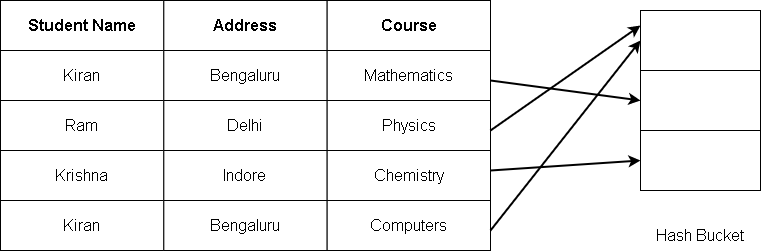
The name and the student address serve as the key. If two records are similar, they are included in the same bucket, thus, eliminating the duplication.

Sorted Neighborhood Technique for Misspelling Integration

The problem with hash key method is that you go over each record to find the duplicate. If the database is extremely large, then it is time consuming.

The sorted neighborhood technique works on the idea that if records are sorted, it is easier to find duplicates because similar tuples will be next to each other.

1. Identify a set of attributes as key in the table with N tuples.
2. Sort the table based on the key. The key is not unique, but a simple key for sorting data such as ” first 3 letters should be ‘Rav’ “.
3. Once the tuples are sorted, you have to create window of W rows over all N tuples.
4. Merge the duplicate based on some rules (ex. merge names if all other values like age, address, department, etc matches) within the window.
5. If the window size of too small, you may not find some duplicates
6. if the window size if too big then also you may miss duplicates.
7. Make multiple pass until there are no more merges of records.

For example:

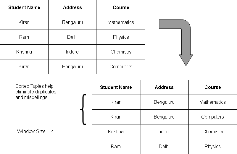
The sorted neighborhood technique ignores misspelled names, omissions in data. The efficiency is solely based on the selection of keys.

Graph-based Transitive Closure to Reduce Number of Passes

This technique answers the question of reducing the number of passes from the sorted neighborhood technique.

• Use sorted neighborhood technique and sort records based on identified keys.
• Create an undirected graph structure where nodes correspond to records and edges corresponds to “is a duplicate of ” relationship.
• Record R1 and R2 need not be compared in any pass if they belong to the same connected component.

Here is an example:

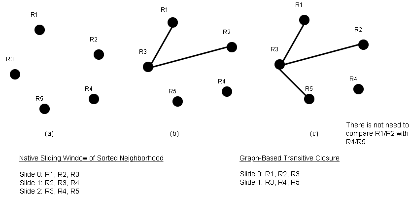
The above diagram clearly shows a reduced number of passes.

In the next article, we will discuss about integrating data into a single schematic structure.

post

Dirty Data And Data Cleaning

The first problem with data mining is that you need proper data. However, it is not possible if we talk about data from different sources. There is a couple of problem when data is from heterogeneous sources and it must be cleaned, transformed into a standard form to be mined. In this article, we will talk about dirty data and data cleaning issues.

The problem with dirty data is listed here.

• Lack of standardization
• Missing, spurious and duplicate data
• Incorrect or Inconsistent data

Lack Of Standardization

Consider internet where data is available in multiple languages, multiple encodings, and locales are available, therefore, there is no common standard with data.

A user may write abbreviation: “Mahatma Gandhi Road” and another one writes “M.G. Road”. Both are same in meaning but there are written in different ways.

Then there is problem of semantic equivalence: “Chennai” is same as “Madras”, “Mumbai” is same as “Bombay”.

Even people use multiple standards such as 1.6 miles is same as 1 kilometer.

Missing, Spurious, and Duplicate Data

Given a form to fill, the users enter information differently. A few people miss some fields such as age.

Incorrectly entered (spurious) values are common. In the relational databases, duplicate data is common, even though database has been normalized.

There are semantic duplication as well. For instance, B.M.Krishna may appear as M.Balakrishna in another data set.

Incorrect or Inconsistent data

Sometimes the user enter codes that are incorrect and has no meaning. For example, using 0/1 instead of M/F to identify gender is incorrect.

Codes that are inconsistent or outdated are not to be used. For example, traveling eligibility ‘ C ‘ denotes ‘III^rd class’ no longer used.

Inconsistent duplicate data: when two data sets are found to belong to same person but have two different information. For example, address information.

Inconsistent association: when sales figures provided by the marketing department do not add up to the total sales figures by the retail units.

Semantic inconsistencies : when user writes Feb 31st, but there is not Feb 31st in the calendar.

Referential Inconsistencies: Rs. 10 million sales reported from a unit that has been closed already.

Issues In Data Cleaning

Now that you know how dirty data look like we must discuss issues with cleaning the data. The process of data cleaning cannot be automated.

The mining process is very much depended on GIGO( garbage in, garbage out) principle. It means the kind of input determine the output of the system. Therefore, unclean data will not produce good results.

We need considerable knowledge that is not explicit and beyond the purview of the warehouse such as metrics, geography, govt policies, policies, etc, to clean the data.

Note that we haven’t discussed about the multiple sources of data, that adds to the complexity. The complexity increases with the history span that is taken up for cleaning.

In the next article, we will discuss the steps taken to clean the data.

post

Operational Database vs. Data Warehouse

In this article, we will evaluate operational database vs. data warehouse. Operational database is live database which uses normalization, concurrency control to manage transactions, and have a recovery mechanism. It is used by OLTP (Online Transaction Processing) applications.

The data warehouse is kept separate from the OLTP databases. It is used by the OLAP( online analytical processing) applications. It is more about summarization and aggregation of data. If applied to a operational database, it will slow down the OLTP system.

Difference Between Operational Database and Data Warehouse

When we say operational database, we actually mean OLTP systems, and data warehouse means OLAP systems. Therefore, in the following table, you find feature-wise comparison of these two databases.

Features	Operational Database	Data warehouse
Users	Clients, Clerks, IT guys	Managers, Executives, Analysts
System Orientation	Customer oriented, data-to-day operation	Market Oriented, Decision support
Data	Current data	Historical data
DB Design	E-R Model	Star or Snow flake Model
View	Focus on current data, same organization	Focus on multiple versions of data, heterogeneous sources
Volume	Not very large	Huge, stored in many disks
DB Access	Short, atomic transaction, ACID property	Read-only access with complex queries
Operations	Index/Hash on Primary key	Lot of Scans
No. of records	Tens	Millions
DB Size	100 MB to GB	100 GB to TB
Priority	High priority	High flexibility
Metric	Transaction throughput	Query response time

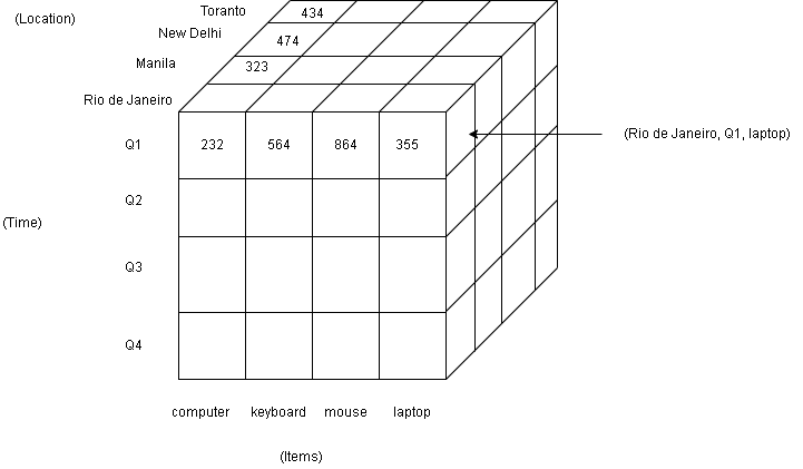
Multi-Dimensional Data Model of Data Warehouse

A multi-dimensional model categories data as

• either facts with numeric measures.
• or as dimensions that characterize the facts and are mostly textual.

For example.

Product sold to customer in certain amount and price

Fact : – purchase

Measures:- amount, price

Dimension:- location, type of product, time of purchase

Multi-Dimensional Model

Multi-dimensional data model is composed of logical cubes, measures, dimensions.

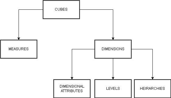
Measures – It populate the individual cells of a logical cube.

e.g. quantity of sales which is some number

Dimension – They are ways to look at the measures. A cube has 3 dimensions. Each of the dimension has cells with some quantity as measures. One dimension may be location,another time, and so on.

Logical hierarchies – They are ways to organize data at different level of aggregation. The members at each level have one-to-many and parent-child relationship.

e.g Quarter-I ( year 2018), Quarter-II (year 2018), Quarter-III(year 2018)

The quarter-i, quarter-ii, and quarter-iii are children of year 2018.

e.g Year -> Month -> Weeks -> Days -> Hours (5 levels)

Sales Target ->Area -> Sales Rep -> Individual Target (4 levels)

The hierarchy and levels have many-to-many relationship.

Logical Attributes – It provide additional information about the data.

Multi-Dimensional Data Storage

The data cube represents all measures. Each dimension is the edge of the cube. They divide the cube into cells containing values or data.

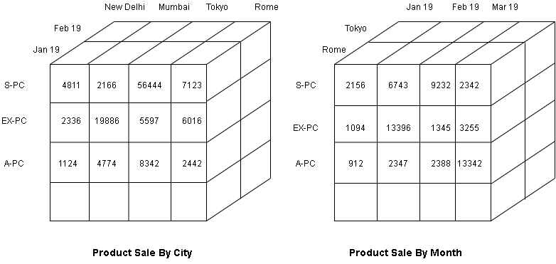
The cube can rotate to give many view of same data. It also represents physical storage of measures, just like relations in OLTP database.

A measure can have more than three dimensions, but pictorially, cube has only 3 dimensions and additional dimensions requires additional cubes.

Schema For Multi-Dimensional Database

The relational implementation of the multi-dimensional data model is a

• A Star Schema
• A Snowflake Schema
• A Fact Constellation Schema

We will discuss the architecture of data warehouse in future lessons. In this article, you learned that the data warehouse is different in all aspects compared to operational database.

post

Data Warehouse Concepts

In this document, you will find all articles related to mining data and data warehouse. We will also briefly discuss about the OLTP and OLAP, data cleaning concepts.

A data warehouse is “a copy of transaction data specifically structured for query and analysis“

Ralph Kimball

• Difference Between OLTP and OLAP
• Operational Database vs. Data Warehouse
• Dirty Data And Data Cleaning
• Steps In Data Cleaning
• Transformation Algorithms
• Integration Of Data Sources In Data Mining

post

Difference Between OLTP and OLAP

In the application world, there are two types of applications from the database perspective. Operational data and Historical data related to OLTP and OLAP applications respectively. In this article, we will you will learn the difference between OLTP and OLAP applications.

Operations Data (OLTP applications)

The operational data are those that “works”. It means these data are frequently updated and queried. The database is normalized for efficient search and updates. Therefore, you will not find update anomalies due to normalization process.

The operational data is stored on disks a typically suffers fragmentation, and it has local relevance. The data affected is in the same location that from a remote source.

The queries are very precise and access individual tuples. Most of them are transactional in nature.

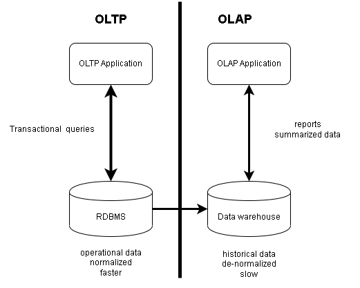
Historical Data (OLAP applications)

Another set of data is historical data, and it “tells” mainly gives “insight”. The updates to a database that store historical information need not update frequently. These are used by OLAP (Online Analytical Processing) applications.

The data is accumulated from several sources, and it has integrated data set with a global relevance.

The queries in such a system are analytical in nature, and therefore, requires huge amount of aggregation. Then there are performance issues during queries, not during updates as in the case of operational database.

Examples Of OLTP Queries

What is the salary of Mr. Mithra?
What is the address and phone no. of the person in-charge of the finance department?
How many people working in engineering department?

Examples of OLAP Queries

How is the employee attrition scene changing over the years across the company?
Is there correlation between the geographic location of a company unit and excellent employee appraisals?
Is it financially viable to continue our manufacturing unit in China?

You can see a clear difference between the nature of queries in OLTP and OLAP. In next lesson, we discuss the dirty data and data warehouse.

post

Kind Of Patterns In Data Mining

Earlier we talked about mining patterns from data repositories. In this article, you will learn about kind of patterns in data mining. The pattern mining are tasks performed by the data mining engine. Later the patterns can be evaluated based on the interestingness measures.

Mining Tasks

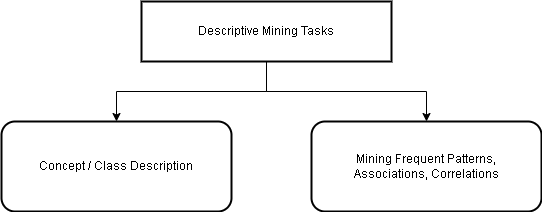
The data mining tasks are classified into two categories – descriptive and predictive.

Descriptive Mining Tasks	This describes the general character or properties of data.
Predictive Mining Tasks	These tasks perform inference on data to make future predictions.

Concept / Class Description

The concept or class description deals with the task of characterization and description of data. Data can be associated with classes or concepts. For example,

Classes of items for sale include computers and printers

Customer concept include big spender and budget spender which purchasing items.

The classes must be described in clear and concise terms which is known as ” class / concept description “.

How To Find Such Descriptions?

There are three ways to find class / concept description.

Data Characterization – This is summarizing the data of target class based on features.

Data Discrimination – This compares the target class with one or more comparative classes called the contrasting classes.

The third option is to use both data characterization and data discrimination.

What Are The Methods Of Data Characterization ?

There are simple methods to characterize the data. One is simple summaries based on statistical measures. Second is the roll-up operation on OLAP data cube that also summarizes the data. The third method is to use the attribute oriented induction technique.

The output of characterization can be presented in various forms. For example, Pie Charts, Bar Charts, Curves, Multi-dimensional data cubes and multi-dimensional tables.

The resulting descriptions can also be presented as generalized relations or in rule form called characteristic rules.

Data Characterization Example

Q1. Produce a description of summarizing the characteristics of customer whole spend Rs 3000 in last 6 months.

The result could be a general profile of customers such as 40-50 year old, employed, credit rating and other features.

Data Discrimination Example

Q2. Compare features of software products whose sales up by 10 % in last year with software product whose sales went down by 30%.

The resultant description is same as that of data characterization, however, we also have comparative measures that distinguish the target class and contrasting class.

Mining Frequent Patterns, Associations, and Correlations

The frequent patterns are those patterns that occur frequently in data. The frequent pattern includes frequent item sets, sub-sequences, and sub-structures.

Frequent Item-set

Those items that frequently appear together in a transactional data set is called frequent item-set.

Frequent Sub-sequence

The customer buying first PC, then camera, then a memory card is an example of sub-sequence.

Frequent Sub-structure

The sub-structure means different structural forms such as graphs, trees, and lattices, that are combined with item-sets and/or sub-sequences.

Association Analysis

Association analysis identify relationship between items that are bought together during transactions. Consider the following example.

Example: A store want to known which is purchased together. So they created rules such as 

buys(X, "computer") => buys(X, accessories") [support = 1%, confidence = 50%]

where X is the customer, the confidence or certainty is 50% means if X buys computer, there is 50% chance that he will buy computer accessories. 

Support means of all transaction % is where computer and computer accessories bought together.

Consider another rule like above.

age(X, "20 ... 29") And income(X, "20K ... 29K") => buys (X, "CD Player") [support = 2%, confidence = 60%]

The second rule is example of multi-dimensional rule where more than two attributes – age and income are involved.

Therefore, frequent item-set mining is the simplest form of frequent pattern mining.

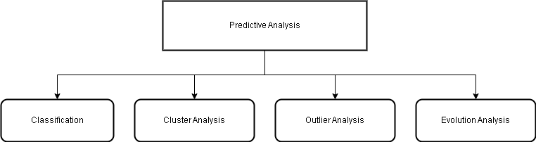
Classification

There are many predictive analysis techniques which extract information from the data to make predictions about future results. Classification is the process of finding a model or function that

• describe and distinguishes data classes or concepts
• for using the model to predict the class of objects
• whose class label is unknown.

In short, use the existing data of classes or concepts and create a model that predict for object of unknown classes.

This model analyze training data ( data of known classes) to build the predictive model.

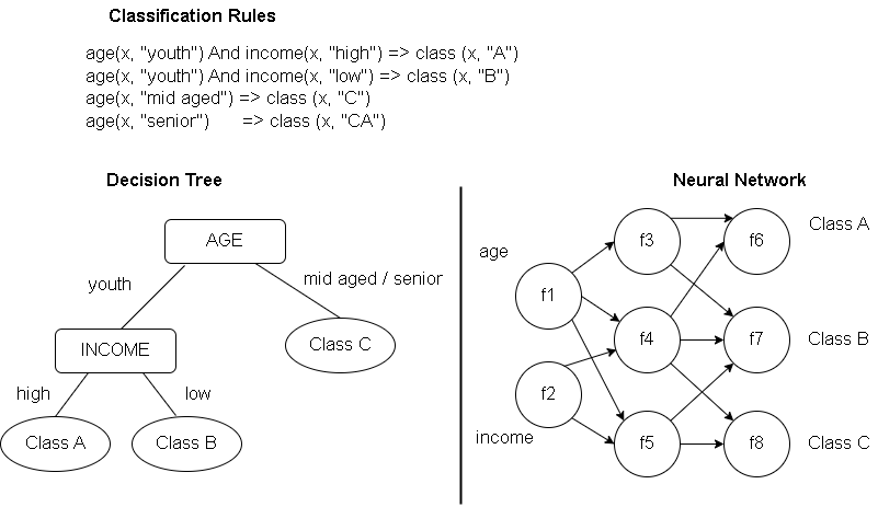
How This Model Presented ?

There are three different ways to present this model.

• classification rules
• decision trees
• mathematical formulae or neural networks

The neural network is collection of neurons like processing units with weighted connections between the units.

The classification algorithms find relationships and predicts categorical (discrete, unordered) labels for classes. However, if the prediction model is continuous-valued functions. If does numerical predictions and give numerical values, not class labels.

A regression analysis is done in such cases.

Examples:

Q. To classify a large set of items in the store, based on 3 kinds of responses to a sales campaign : good, mild, and no response.

So, we can target these three classes and make a model for these classes based on the features of the items, such as price, brand, place made, type and category. These features are predictors and the data is used for classification in future.

Cluster Analysis

The cluster analyze data without consulting a known class label. The objects are clustered based on principle of maximizing the inter-class similarity and minimizing the inter-class similarity.

Objects are similar in one cluster, but dissimilar to objects in other cluster.

Outlier Analysis

Data objects that do no comply with the general behavior or model of the data. These data are outliers.

Most mining methods discard outliers as noise or exceptions.

Mining of outliers known as outlier mining. Sometimes useful in fraud detection to people who are interested in rare events.

Some examples are – extremely large purchase, fraudulent usage of credit cards, etc.

Evolution Analysis

The data evolution analysis describes and models regularities or trends for objects whose behavior changes over time.

Example:- correlation, clustering of time-series data.

We have seen patterns types, but patterns are interesting only is they are useful, easily understood by humans, novel in nature, and valid on new or old test data with some certainty.

Some interesting patterns are based on subjective measures such as user belief. The patterns thus discovered must lead to some action or confirm some hypothesis. Therefore, you keep in mind that all minded patterns are not interesting.

post

Kind of Data In Data Mining

Data mining uses a variety of techniques from multiple disciplines such as statistics, machine learning, high performance computing, pattern recognition, neural networks, data visualization, signal processing, and image processing. In addition to this, we must learn the kind of data in data mining.

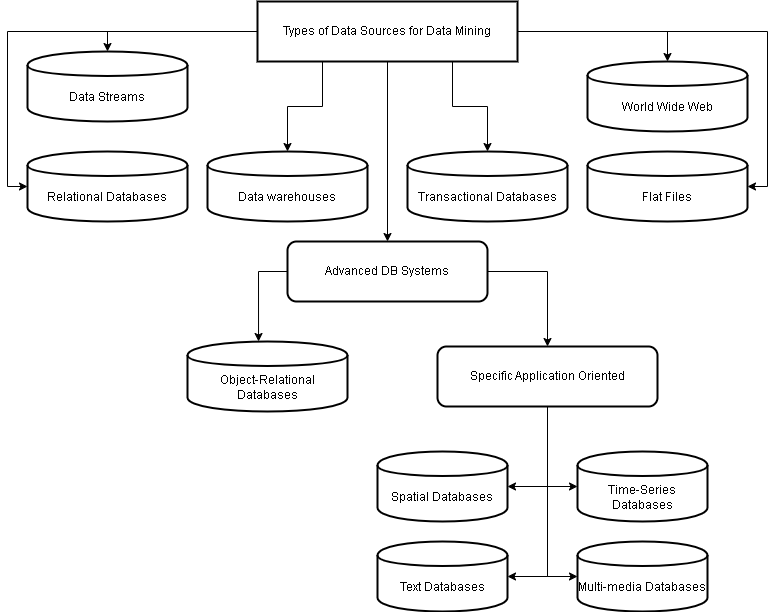
Data Sources

Data mining is applied to all kinds of databases including data streams and web. Here is a list of data sources supported by data mining technologies.

1. Relational databases
2. Data warehouses
3. Transactional databases
4. Advanced database systems
5. Flat files
6. Data streams
7. World Wide Web

Each of the data repository requires different techniques. In the rest of the article, we will discuss about each database and give an overview of the database systems.

Relational Databases

The relation database is also known as RDBMS ( relational database management system). It is a collection of databases connected via relationships. The relational database consists of tables known as relations with columns and row. The columns are attributes or field and the row are tuples or records.

The tuples are identified uniquely by a set of keys.

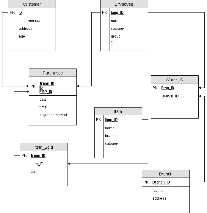
The relational database starts with a semantic model of database called E-R Diagram. For example, let us create a new relational database for ITStore – a fictitious company that sell computer and its accessories.

The first step is to create define the schema for relations in the database.

Customer(ID(key), customer name, address, age, occupation, annual income, credit information, category)
Item(Item_ID(key), name, brand, category, type, price, place made, supplier, cost)
Employee(Emp_ID(key), name, category, group, salary, commission)
Branch(Branch_ID(key), name, address)
Purchase(Trans_ID(key), ID(key),Emp_ID(key),date,time, payment method,amount)
Item_Sold(Trans_ID(key), Item_ID, qty)
Works_At(Emp_ID(key),Branch_ID)

The next step is to create relations and set relationships between them such that we can query the database using SQL and get results.

The query is transformed into relational operators such join, selection, and projection and is then optimized for efficient processing.

The relational queries uses aggregate functions such as sum, avg(average), count, max(maximum) and min(minimum).

Data mining on relational database search for trends or data patterns. For example, in the about relational database, based on customer income, age, and credit information we can find credit risks for new customers.

We can also compare sales of current year from the sales of previous year etc.

Data warehouses

Consider the previous example of ITStore, if the CEO of the company want to know “Sales of each item” at “each branch” for “last 6 months”. Since, the data is located at different branches it is difficult task to analyze the data.

However, if ITStore has a data warehouse the task would have been easy. The data warehouse is a single repository that has data from many sources under a unified schema.

A data warehouse is constructed via a process of

1. data cleaning
2. data integration
3. data transformation
4. periodic data refreshing

The data in the data warehouse is stored around major subjects such as

customer, sales, items, suppliers, etc.

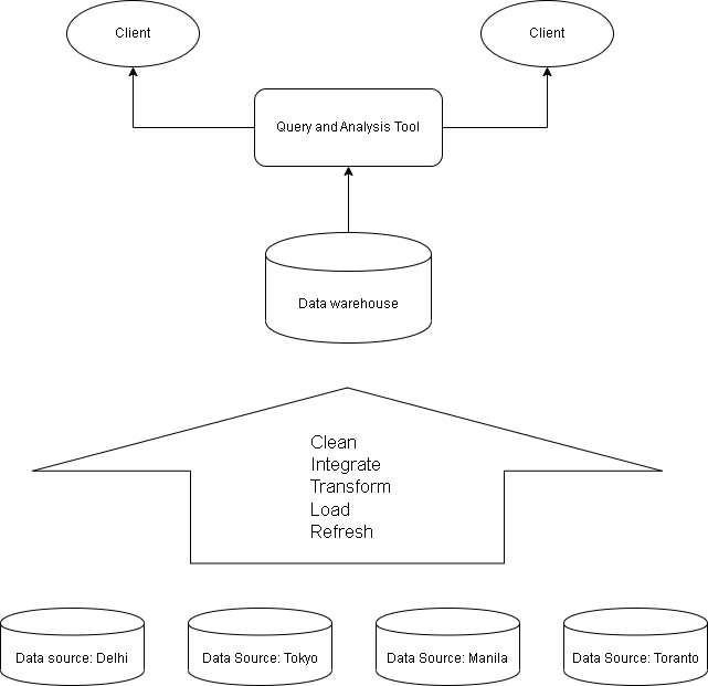
These data is stored to provide information from historical perspective (5 – 10 years of data) and are summarized.

A data warehouse is modeled by multi-dimensional database structure where each dimension is an attribute or set of attributes in the schema, each cell stores some values of some aggregate measure such as count, or sales amount.

The physical structure of the data warehouse is a data cube or relational data store.

Transactional Databases

A transactional database consists of file where each record represents a transaction. Each of the transaction has transaction id and list of items involved in the transactions.

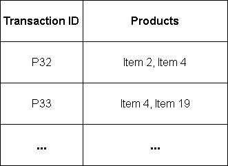
Data mining on transactional database many answer queries like “Which items sold well together? “

We can answer the query by looking at set of items sold together frequently.

Advanced Data And Information Systems

Advanced data and information systems are required by some modern applications that handle

• Maps (spacial data)
• IC Circuit Design, Building Design ( engineering design data)
• Text, audio, video, images (html and other multi-media)
• Historical facts, stock exchange data ( time based data)
• Sensor data, CCTV recordings (stream data)
• Internet data (world wide web)

There are many advanced databases to handle such data types. They are

• Object-Relational Database
• Spatial Database
• Temporal Database
• Spatial-temporal Database
• Text and Multimedia Database
• Heterogeneous and Legacy systems
• Data stream management systems

At this moment we step discussing about the databases. In future articles, we will explore each of the databases in-depth.

post

Data Mining Architecture And Its Components

We now discuss the data mining architecture and its components. We will learn about the functionality of each component and its role in the data mining system.

These are the components that found in a typical data mining system. In some systems, the components are integrated into one, however, the functionality is different at different time with data sets.

Databases and Data warehouse

The databases, data warehouse, world wide web, and other repositories are one or more set of databases on which data cleaning, data integration is performed.

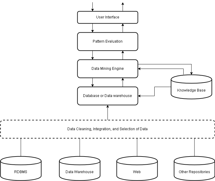
All information is stored in database servers or data warehouse server responsible for fetching relevant data based on user’s data mining request.

Domain Knowledge Base

The domain knowledge base guide the search or evaluate the interesting patterns in the result of a data mining query. There are knowledge such as concept hierarchies that explore different types of hierarchical relationships in data. The attributes and values are organized into different levels of abstraction. e.g schema hierarchy.

There is also user beliefs in evaluating the patterns . A set of belief is used to compare with the result e.g unexpectedness.

Data Mining Engine

Each domain has specific problems that you want to solve, for which you need to run data mining tasks. But this process is not so easy. You need knowledge of domain and identify which tasks are suitable in solving those problems.

The data mining engine does the data mining tasks using a set of functional modules. The tasks are

1. characterization
2. association
3. correlation analysis
4. classification
5. prediction
6. cluster analysis
7. outlier analysis and
8. evolution analysis

There are tools such as KIRA that can guide you through the data mining tasks identification process based on your domain.

Pattern Evaluation Module

The pattern evaluation module interacts with the data mining modules and focus the search towards only interesting patterns. It basically filter out discovered patterns using some interestingness measure.

The pattern evaluation module is sometimes integrated into the data mining modules depending on the mining method you are using.

User Interface

This is a separate module that communicates between the users and the data mining system. It allows users to

• specify data mining query
• providing information to guide the search
• exploratory data mining on intermediate results
• browse, visualize the database and data warehouse in different forms.

The data mining can be viewed as advanced stage of OLTP from data warehouse perspective. Therefore, the data analysis system should handle large amount of data, otherwise, it can be termed something smaller as machine learning system that uses AI, or some statistical data analysis tool, or experimental system.

You must have heard about Big Data. It only mean huge amount of data and nothing else. It define the huge data using 5 V’s – volume, variety, veracity, and velocity.

The data mining on contrast work on large data and extract interesting information.

post

What Are the Steps in Data Mining

In the previous article, you learned the purpose of data mining, which is to help various organizations, including businesses in extracting meaningful information. We are ready to discuss “What are the steps in data mining?”

In the data mining process, each step does some tasks to make the mining process easier. We shall look into each one of them one by one.

Step 1: Data cleaning

The first step is to remove any inconsistencies or noises from the data. This is wants data to be of same standards and be consistent on that standard.

Step 2: Data Integration

If you have multiple sources data, then all the data sources must be combined.

Step 3: Data Selection

Since, there are huge amount of data it is not necessary to read all data for analysis, instead we can only select relevant data such as based on time period, area, department, categories, so on for analysis task.

Step 4: Data Transformation

The data is consolidated or transformed into suitable form for mining.

Step 5: Data Mining

In this important step we use intelligent methods including statistics to extract meaningful patterns from the data.

Step 6: Pattern Evaluation

The patterns extracted that represent some knowledge must be evaluated. There are many interesting measures to evaluate such knowledge.

Step 7: Knowledge Representation

The ultimate goal of data mining is to present the information to users. In the last step, visualization techniques are used to present the mined knowledge to its users.

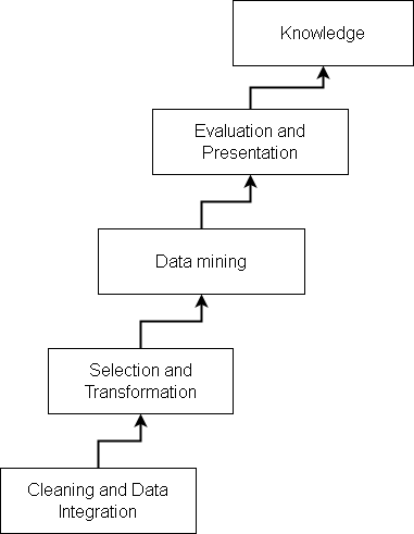
Note that the first four steps – data cleaning, data integration, data selection and data transformation are to prepare data for mining.

post