Data Structures Notes – Concepts, Examples, and Exam-Ready Revision

Data Structures are a core subject in Computer Science and Information Technology (IT) curricula, as well as in competitive examinations such as GATE, UGC NET, and university semester exams.

On this page, you will find structured resources to learn data structures concepts, along with clear explanations, examples and exam-ready revision notes.

What Will You Learn

On this page you will find:

• Core Data structures concepts explained clearly and systematically
• Exam-oriented explanations supported with relevant examples
• MCQ-based practice posts to test your understanding
• Detailed articles along with exam-ready revision PDFs

This Page is for:

• Computer science and IT students
• GATE and other competitive exam aspirants
• University exam preparation
• Self learners who want to revise data structures knowledge.

Topic Sections

Find Data Structures topics here.

(1) Introduction to Data Structures

Data Structures Introduction

(2) Linear Data Structures

Stack
Queues
Queue Basic Operations
Linked-Lists

(3) Non-Linear Data Structures

Tree Basics
Binary Tree Concepts
Binary Tree Operations
Ordered vs. Unordered Tree

(4) Applications of Data Structures

(A) Stack Applications

Tower of Hanoi
Implement Stack in C
Stack using Linked-List
Evaluating Postfix Expression
Infix to Prefix Expression
Infix to Postfix Expression

(B) Queue Applications

Multilevel Queue
Implement Queue using Pointers
Implement Queue using Arrays

(C) Linked-List Applications

Implement Doubly Linked-List
Sum of N numbers using Linked-List

Data-structure – Ordered Tree vs Unordered Tree

A binary tree can be ordered or an unordered tree, so what is the difference between these two trees. In this lesson, you will compare the ordered tree vs. unordered tree and tell the difference.

Ordered Tree Example

The name suggests that the ordered tree must be an organized tree in which nodes are in some order. What is the common ordering method?

In the figure above, for any node, its left child has less value than the node itself and the right child has a value greater than the node.

Unordered Tree

In a binary tree, when nodes are not in a particular order it is called a unordered tree.

See the root, all the left descendants of the root are less than the root value and all right descendant has a value greater than the root.

This is the primary difference between the ordered tree vs. unordered tree.

References

R.G.Dromey. 2008. How to Solve it by Computer. Pearson Education India.

Robert Kruse, Cl Tondo. n.d. Data Structures and Program Design in C. Pearson Education India.

Thomas H. Cormen, Charles E. Leiserson, Ronald Rivest, Clifford Stein. 2009. Introduction to Algorithms. MIT Press.

Data Structure – Binary Tree Concepts

A binary tree is a special kind of tree and important in computer science. There is plenty of real-world application of binary trees. The scope of this lesson is limited to the learning the binary tree concepts.

Learn Tree Basics

Informal definition

A tree is called a binary tree if it has the following properties.

• It is an empty tree with no nodes.
• The tree has a root node, left sub-tree and right sub-tree.
• The sub-trees are binary tree themselves.

Strictly Binary Tree

Suppose there is a binary tree with right sub-tree and left sub-tree. The sub-trees are in turn non-empty, then such a binary tree is called a strictly binary tree.

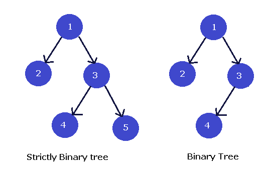
In the above figure, one is a strictly binary tree and the second tree is not a strictly binary tree, but it is certainly a binary tree and satisfy all the properties of a binary tree.

Complete Binary Tree

A complete binary tree has a level L and all its leaf nodes are available at level L. At each level the complete binary tree contains 2^Lnodes.

Let us show this with an example,

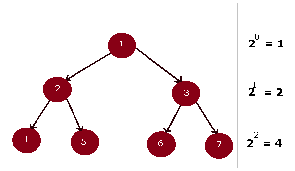
The root is at level 0, therefore, L = 0 and 2^L = 2^0 = 1.

Conversion of a Binary Forest into a Binary Tree

Suppose we have a forest with two trees as follows,

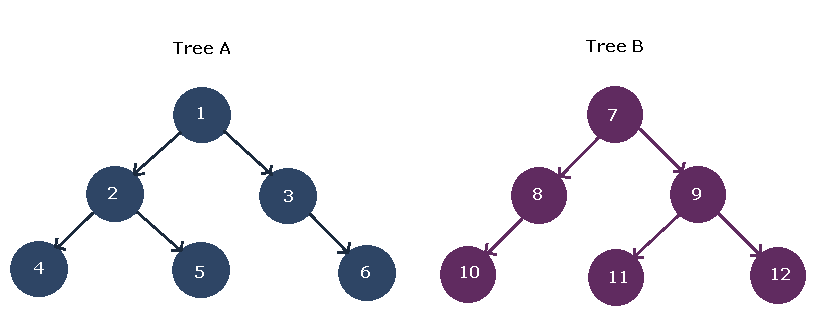
\begin{aligned}
&T1 = { 1,2,3,4,5,6}\\
&T2 = { 7,8,9,10,11,12}
\end{aligned}

The figure below show the two separate trees  in the forest.

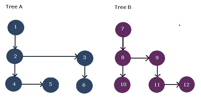
The first step is to order the nodes of both trees using following formula.

• If a node has left child, then if comes immediately below the node.
• If a node has another node in the save level, then it becomes the right child of the node.
• If a node has right child then, ignore it.

Such a representation of two trees is given below.

Your next step should be to join these two tree into one by connecting their roots. This is because the roots of the trees are at the same level. See the figure below

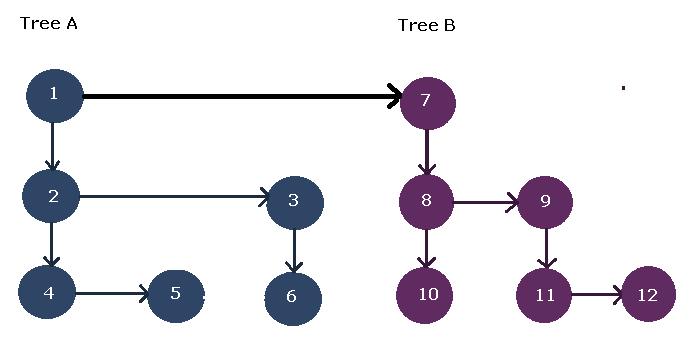
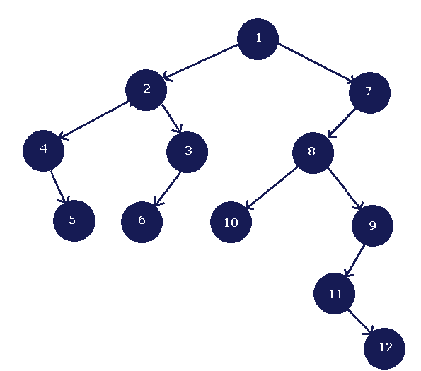
The new tree is a binary tree, the node at the save level in above diagram becomes the right child. The final tree structure look like the one in figure below.

Total Number of Edges

In a complete binary tree, the total number of edges is given by the formula,

\begin{aligned}
2 (N_L - 1)\hspace{1ex} where \hspace{1ex}N_L\hspace{1ex} is \hspace{1ex}total\hspace{1ex} number \hspace{1ex}of\hspace{1ex} leaf \hspace{1ex}nodes.
\end{aligned}

For example, see the tree below.

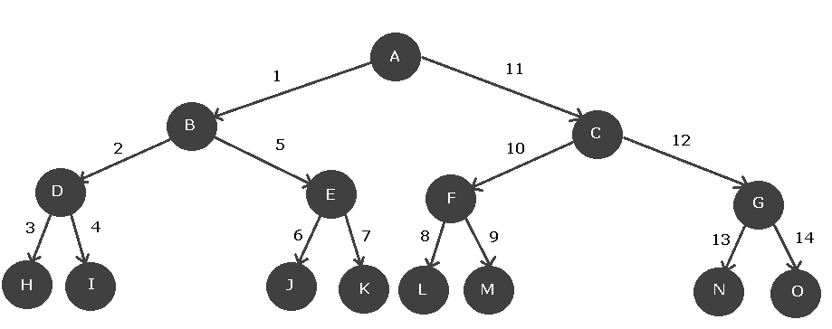
In the above diagram, we have .

Therefore,

\begin{aligned}
&= 2( N_L - 1) \\
&= 2 ( 8 - 1) \\
&= 2 (7) \\
&= 14\hspace{1ex} edges.
\end{aligned}

Height of a Binary Tree

The maximum level of any node of the binary tree is called the height of a binary tree.

For example, see the figure below.

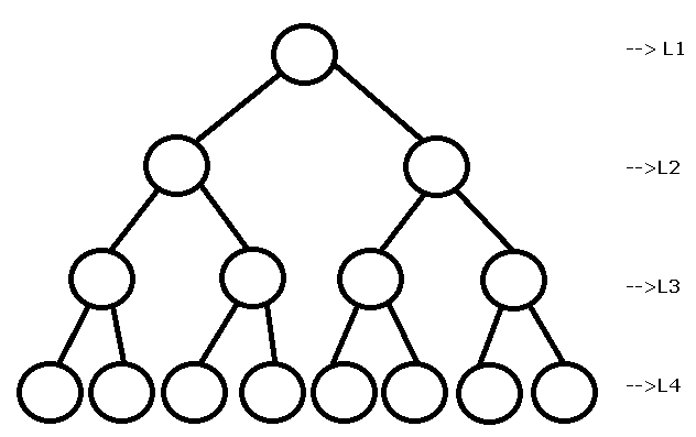
In the above tree figure, the maximum level of the tree is ,

Therefore, the height of the tree is .

References

R.G.Dromey. 2008. How to Solve it by Computer. Pearson Education India.

Robert Kruse, Cl Tondo. n.d. Data Structures and Program Design in C. Pearson Education India.

Thomas H. Cormen, Charles E. Leiserson, Ronald Rivest, Clifford Stein. 2009. Introduction to Algorithms. MIT Press.

Data Structure – Tree Basics

A tree is a non-linear data structure. It means you cannot access an element of a tree in a straightforward manner. In this lesson, you learn about tree basics.

This will serve as a foundation for future topics on trees. You can start learning about other topics if familiar with the basics.

• Learn Binary Tree Concepts
• Learn Binary Tree Operations

Informal definition of Tree

A tree is a set of one or more nodes with a special node called a Root node. Every none points to a left node and a right node. Sometimes left, right or both are missing and a node points to nothing.

Every node is part of some smaller set of nodes called a Sub-tree. Each sub-tree has more sub-trees.

Tree basics – Directed vs Undirected Tree

In an undirected tree, the edge between two nodes has no direction associated with it. However, a directed tree has some important properties.

• The directed tree is acyclic means there is loop between the nodes.
• The directed tree is digraph means it is like a graph with direction. Each node has associated edges. If the node pointed by some other node, it is called an In-degree and if the node is pointing to some other node, its called an Out-degree.
• Root node has in-degree 0 and all other nodes have in-degree of 1.
• The minimum number of nodes allowed in a directed tree is 1. So, an isolated node is a directed tree.

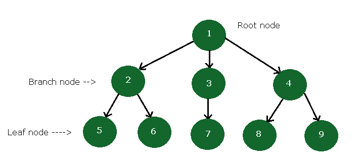
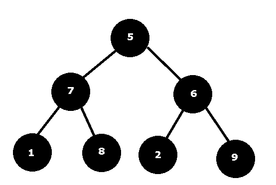
Leaf Nodes

In a directed tree with nodes that has an out-degree of 0 is called a Leaf node or Terminal node.

In the above figure, 5, 6, 7, 8, 9 are leaf nodes.

Branch Nodes

In a directed tree with all nodes other than root and leaf nodes are called Branch nodes. For example,

In the above figure, 2, 3 and 4 are branch nodes.

Level of a Tree

Suppose you want to reach the node 8 from root node 1, then starting from root node, we go through following path

1 –> 4 –> 8

So, the level of any node is length of its path from the root node. The level of root node is 0 and level of node 8 is 2.

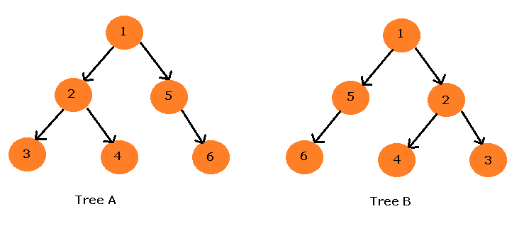
Tree basics – Ordered Tree

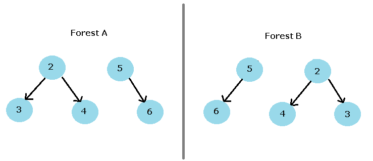
Sometimes the directed tree is ordered, that is, at each level the order is specified, and this type of tree is called an Ordered tree.

In the above figure, the Tree A and Tree B are the same tree but ordered differently.

Node degree

The node degree corresponds to number of children of the node. The node 3,4,and 6 in tree A are leaf nodes and has a degree of 0 because it not a parent of any other node.

The node 2 from tree B has a degree of 2 because node 4 and node 3 are its children.

The Concept of Forest

If we delete root node and its edges from tree A or tree B, we will get two separate trees. This particular set of trees is known as a Forest.

For example, we get the following forest after deleting the root. These forest can be represented as sets.They are the same sets.

Forest A ={ (2,3,4),( 5,6)}                                     Forest B = {(5,6),(2,3,4)}

Descendant and Children of a Node

There is a node called S and it is reachable from node N means there is a path from N to S. Then an such node S is called a Descendant of a node N.

Suppose a node S reachable by a single edge E from node N is called a Child of node N and the node N is a Parent of child node S.

For example, In Tree A

The node 2 and node 5 are children of node 1

The node 3 and node 4 are not children, but descendant of node 1.

Note: We will be using this tree basics terminology in all future lessons. Make yourselves familiar with the concepts.

References

E.Balaguruswamy. 2013. Data Structures Using C. McGraw Hill Education.

Thomas H. Cormen, Charles E. Leiserson, Ronald Rivest, Clifford Stein. 2009. Introduction to Algorithms. MIT Press.

Stack

Stack is a linear data structure that is widely used in operating systems and many applications. The stack implies an office stack of files in which you put new files on the top and the employee always take care of the newly arrived file first.

Similarly, when a stack is implemented in whichever method you want it to, newly elements are added to or deleted from the top of the stack, and stack operations always take the top elements and work its way downwards until the stack is empty.

Two ways to implement a stack are:

1. Arrays
2. Linked Lists

How does a Stack Works

Stack follows a principle called Last in, First Out or LIFO.

The elements are added to the top or deleted from the top using stack operations.

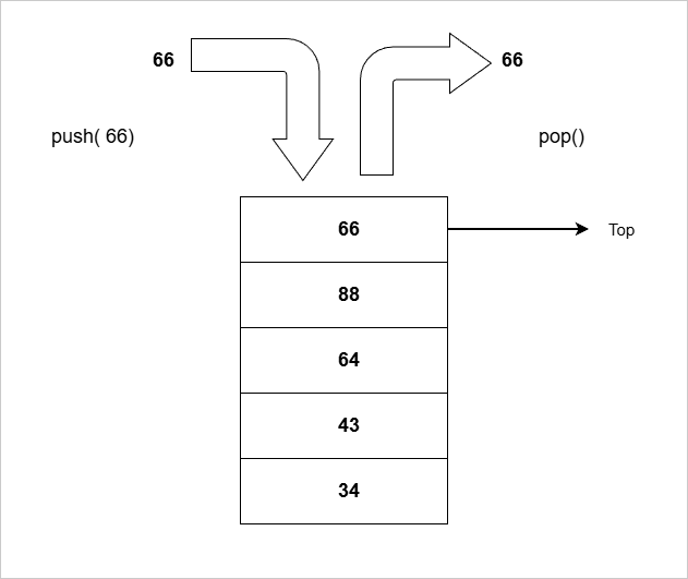
In the figure above, we inserted a number 66 at the top of the Stack with push(66); method. When we want to delete from the stack, we can’t delete anywhere from the Stack. We can only delete element at the top of the Stack which is number 66.

To delete from the top, we can use pop(); method. The pop() does not take any parameters, it simply delete top of the Stack element.

Stack Operations

Stack operations are methods or functions that can add, delete or check status of stack. Here is a list.

1. push();
2. pop();
3. peek();
4. isEmpty;

Push()

This function or method will insert an element to the top of the Stack.

Suppose our stack is

let stack = [23, 44, 66];
stack.push(77);
console.log(stack);

Pop()

This function deletes the topmost element from the Stack.

Suppose for a given stack.

stack = [43, 64, 88];
stack.pop();
console.log(stack); // returns [43, 64]

Peek()

This returns the topmost element of the start with any modification. It is just to display or get the top of the stack element.

stack = [20, 30, 40];
stack.peek();
print(stack);// returns 40 

isEmpty()

The isEmpty() method is to check whether stack is empty of not. It will return a Boolean value.

stack = [44, 88];
value = stack.isEmpty();
console.log(value) //returns False because stack is not empty.

Note: all code examples are in JavaScript and only push() and pop() are built-in functions.

How to Implement Stack in JavaScript

class Stack {
  constructor() {
    this.items = [];
  }

  push(element) {
    this.items.push(element);
  }

  pop() {
    if (this.isEmpty()) {
      console.log("Stack Underflow");
      return null;
    }
    return this.items.pop();
  }

  peek() {
    if (this.isEmpty()) {
      console.log("Stack is empty");
      return null;
    }
    return this.items[this.items.length - 1]; // Access the last element
  }

  isEmpty() {
    return this.items.length === 0;
  }

  size() {
    return this.items.length;
  }
}

// Usage example
const myStack = new Stack();
myStack.push(10);
myStack.push(20);
console.log(myStack.peek()); // Output: 20
myStack.pop();
console.log(myStack.peek()); // Output: 10

Applications of Stack

Here I give you some programs to implement stack to solve a programming problem in different programming languages.

• Tower of Hanoi
• Implement Stack in C
• Implement Stack using Linked List
• Evaluating Postfix Expressions
• Convert Infix to Postfix Expressions
• Convert Infix to Prefix Expressions

Tower of Hanoi

The Tower of Hanoi game is very useful in understanding the recurrence relation. The recurrence relation is a mathematical formula that define a sequence.

Each term of the sequence is found by applying the formula to one or more previous terms. It also requires initial values to start the sequence.

Let’s understand the working of Tower of Hanoi which is a recurrence relation.

The Rules for Tower of Hanoi

It is a game of moving N disk between 3 needles. However, there are some rules we must follow before moving a disk from one needle to second needle.

Rule 1: Move only one disk at a time and it must be a top one.

Rule 2. Cannot move a larger disk on top of smaller one.

Rule 3: Number of moves should be minimum.

Let see how this works for 3 disk Tower of Hanoi game and using output of the game we can find solution to Tower of Hanoi game for N disk.

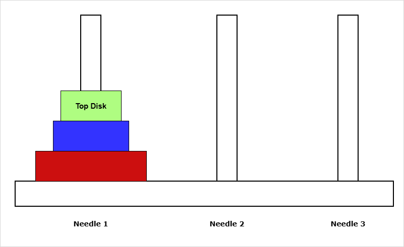
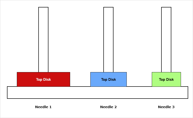
Initially , our disks stacked in needle 1 and other two remain empty. Each time we move a disk it is counted as 1.

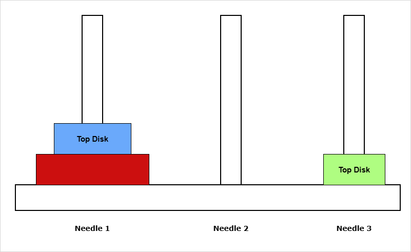
Move top disk from needle 1 to needle 3.

Move top disk from needle 1 to needle 2.

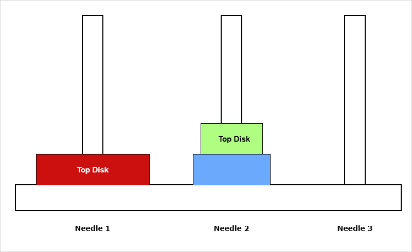
Move top disk from needle 3 to needle 2.

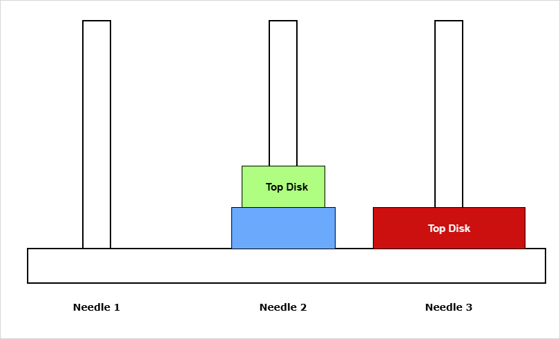
Move top disk from needle 1 to needle 3.

Move top disk from needle 2 to needle 1.

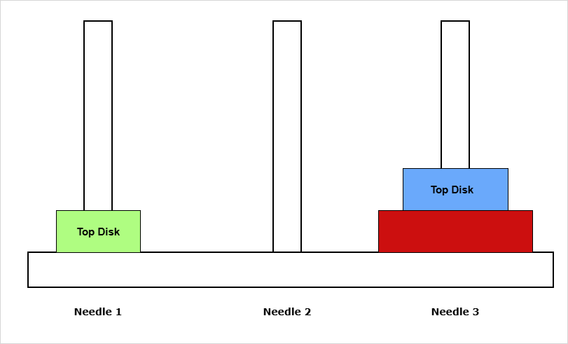
Move top disk from needle 2 to needle 3.

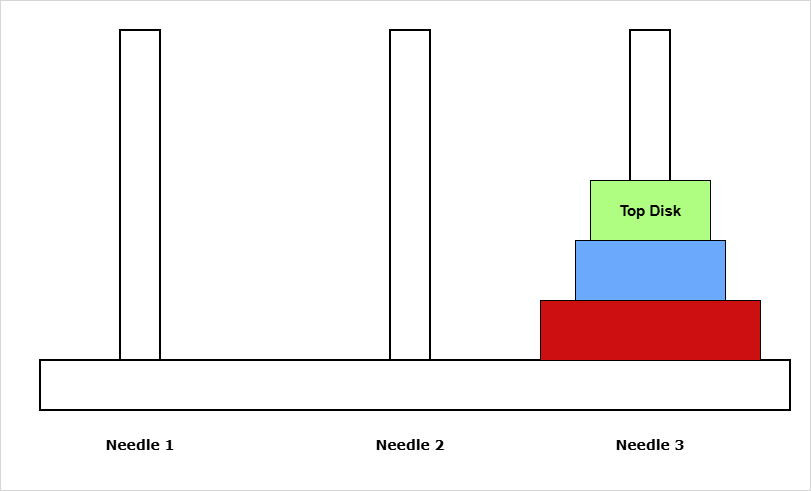
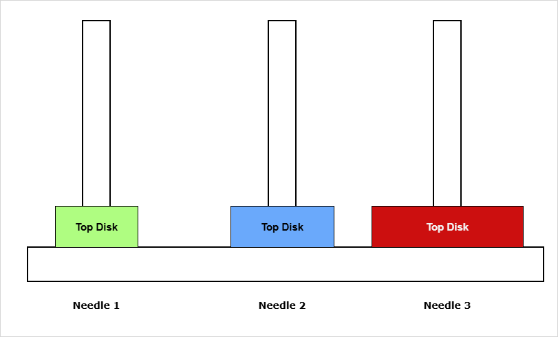
Move top disk from needle 1 to needle 3.

It took total 7 moves to shift all 3 disks to the destination(Needle 3).

Computing for 4 Disk Tower of Hanoi Game

Let the total number of disk move be H.
If we want to compute total count for 4 disk Tower of Hanoi game.

H_{n} = 2(H_{n-1})+1\\
= 2 (7 ) + 1\\
= 14 + 1
= 15 \hspace{3px} moves

There minimum 15 disk move required for 4 disk Tower of Hanoi game.

We can derive a much easier formula for  H_{n}=2(H_{n-1}) +1

H_n = 2^n - 1

How we arrived at this solution, we leave it as an exercise for you.

Queue

A Queue is linear data structure that stores data in a specific order. Insertion in a queue happens at rear-end and deletion at the front-end of the queue. It follows First In, First Out ( FIFO ) principle which means the first element is the one that gets deleted first , because all other elements are added at the rear-end of the queue.

Key Characteristics of Queues

1. Linear data structures.
2. The order of insertion and deletion is specific.
3. Restriction in accessing elements of queue, insertion is at rear and deletion from front.
4. Random access to any element in the queue is not possible.

Why Queues are Useful Structures

Queues are useful when you want tasks to complete in an orderly and predictable manner.

1. It organize task processing in sequential manner.
2. Fair resource allocation because resources like CPU, Memory, Printer, etc., are assigned in order so that no newer process can jump ahead. The resource allocation is predictable.
3. Algorithms like Breadth First Search (BFS) use queue structures.
4. Queue is used in OS CPU scheduling, control the flow of data packets in networking, and more.

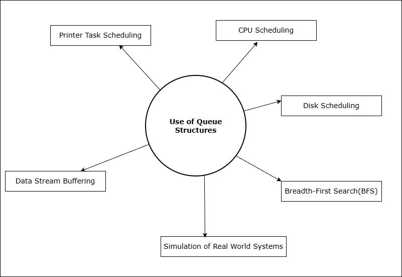
When to Use a Queue

A queue is useful data structures to use when tasks must be processed in the same order they arrive. In other words, if you need to handle tasks in a fair , predictable and sequential order , a queue is the best choice. A queue is frequently used in following scenarios:

1. CPU Scheduling
2. Disk Scheduling
3. Breadth-First Search (BFS)
4. Simulation of Real-World Systems
5. Data Stream Buffering
6. Printer Task Scheduling

CPU Scheduling

The CPU Scheduling is part of operating system that decide which process should be assigned to CPU. The main task of CPU Scheduling is to reduce idle time for CPU and no process should starve while waiting for CPU time.

It uses

1. Multiple queues to manage processes.
2. Scheduling algorithms to increase the efficiency of CPU.

What are the different queues used by CPU scheduling?

1. Job Queue – All new processes goes into the job queue.
2. Waiting Queue – All processing waiting for some resource like printer, some data, etc., are scheduled in the waiting queue.
3. Ready Queue – All processes waiting for CPU time are queued in the ready queue, but allocated according to one of the CPU scheduling algorithms – FCFS, SJF, Round-Robin , Priority Scheduling, SRTF and Multi-level Queue.

Disk Scheduling

The disk scheduling uses a queue to manage all pending I/O requests from processes. When a process makes an I/O request it has three information.

1. Track number of the request.
2. Type of operations – read/write.
3. Process that made the request.

The goal of the disk scheduling is to minimize the seek time and improve the performance. The disk controller can handle only one request at a time. So the entire scheduling process is:

1. Collect all pending requests and put them in a queue.
2. Use Disk scheduling algorithm to send the next job to the disk controller. The most common disk scheduling algorithms are: FCFS, SSTF, SCAN, LOOK, and C-LOOK.

Breadth-First Search (BFS)

The breadth-first-search uses a FIFO queue to process nodes of a graph for searching the key element. It employs a simple strategy.

1. Start with a source node.
2. Node visited , enqueue it.
3. Dequeue the front of the queue.
4. Visit all the neighbors.
5. For each neighbor, repeat step 2-4

Simple example

Consider a graph as shown in following figure.

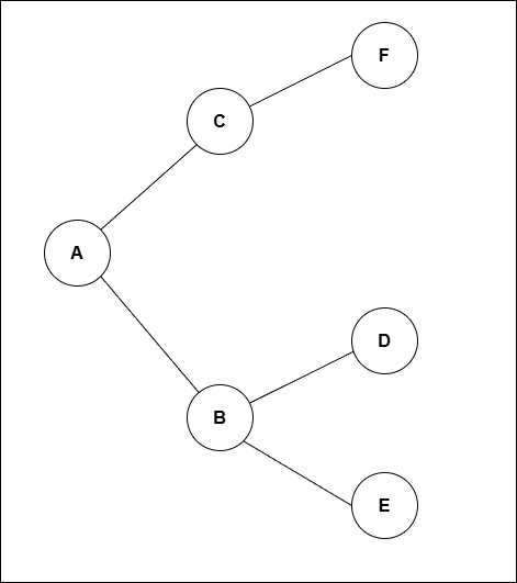
Step1:

Start -> Enqueue (A).

Queue -> [A].

Step2:

Dequeue (A) -> Visit neighbors B,C.

Enqueue (B, C).

Queue -> [B, C]

Step3:

Dequeue (B) -> Visit neighbors D, E.

Enqueue (D, E).

Queue -> [C, D, E]

and continue the process until you have found the search key.

Simulation of a Real World System

The simulation of a real world system is a computer-based model. It imitates the behavior of the real world system under different conditions. This helps researchers to study the performance, make predictions, and make decisions without affecting the real world system.

Some Examples of Simulation

1. Simulating a bank to understand, how many counters required to reduce the wait time. This model use to study – customer arrivals, service time required, and number of tellers.
2. Flight simulator is used to train pilot for difficult situations like engine failure during flight.
3. Weather simulator that can predict the path of a hurricane.
4. Traffic Simulator that can evaluate the effect of a flyover at a busy junction.

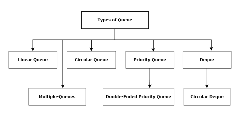
Types of Queues

• Linear Queue
• Circular Queue
• Priority Queue
• Deque
• Circular Deque
• Double-Ended Priority Queue
• Multiple-Queues

Frequently Asked Questions (FAQs)

Linked List

Linked list is a linear data structure that uses dynamic memory to construct the list. There are many types of lists. Since, a list is abstract data type its operations are also different from normal builtin types. In this document, you will find articles related to linked-lists.

Linked List Articles

• Singly Linked List
• Inserting And Deleting From Singly Linked List
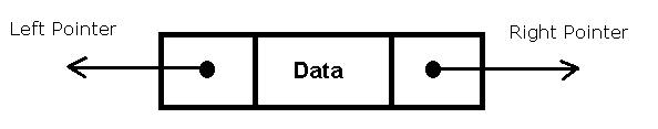
• Doubly Linked List
• Inserting A Node In Doubly Linked List
• Deleting A Node From Doubly Linked List
• Circular Linked List
• Inserting A Node Into Singly Circular Linked List
• Deleting A Node from Singly Circular Linked List
• Concatenating Two Singly Circular Linked Lists

Linked List Examples

• Stack Using Linked List
• Doubly Linked List In C
• Sum Of N Numbers Using Linked List

Queue Basic Operations

Queue is a linear data structure and an abstract data type which is defined using some basic data type in programming languages. A queue data structure is implemented using an array or a linked-list type in a programming language.

There are two pointers that mark both ends of a queue.

• Front
• Rear

A queue works on FIFO principle, First In, First out, any element that goes first must come out first.

There are 3 operations performed on a queue

• Enqueue – insert element at the rear of the queue.
• Dequeue – remove elements from the front of the queue.
• Display – display elements of queue.

Enqueue Operation

The enqueue operation is performed in rear end of the queue. You cannot insert into queue data structure if queue is full. When the queue has space, the enqueue operation insert an element and update the ‘rear’ pointer by incrementing it.

For example

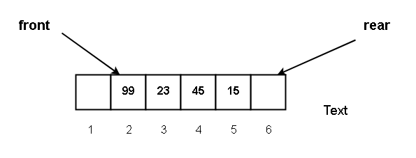
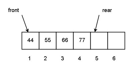
The current status of a queue is given below.

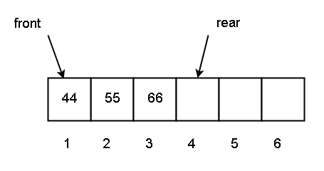
Q [1] = 44 and front = 1, Q [3] = 66 and rear = 4

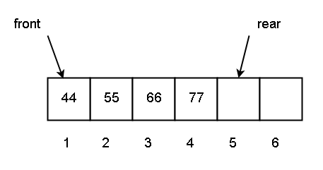
We will insert element 77 at the rear end of the queue, i.e., Q [4] = 77.

new status of the queue after enqueue operation will be following.

Dequeue Operation

Dequeue operation removes an element from the front of the queue. But the queue must not be empty for dequeue operation to work. An element from the front is removed and ‘front’ pointer is updated.

For example

Consider the status of a queue given below

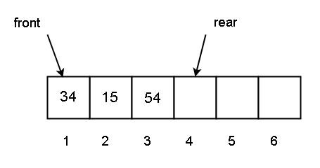
Q [1] = 34 and front = 1

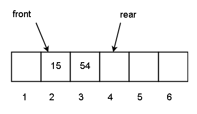
You decided to delete Q [1], after deletion front = 1 + 1 = 2

The current queue is shown in following diagram,

Display Operation

This is a simple operation where we traverse through the entire queue and display the list of elements. This function is the same for both array and linked-list implementation of a queue data structure.

Types of Queues

There are different types of queues data structure about which we will learn in future lessons. The list of queues is given below.

• Circular Queue – where there is not end to the queue and elements are added or deleted in circular motion.
• Priority Queue – elements of queue are in a specific order.
• Double-Ended Queue – queue elements can be deleted or inserted from both ends.

Queue Empty and Queue full Scenario

Before inserting or deleting from queue we must check for two conditions

• Is the queue empty?
• Is the queue full?

Let’s see each scenario in more detail.

Queue Empty Scenario

When queue is initiated both front = rear = 1, but after that when front==rear then it means that the queue is empty and we cannot delete from the queue because that will be an underflow.

For example

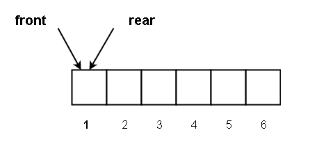
Consider an array based empty queue, where front = rear = 1.

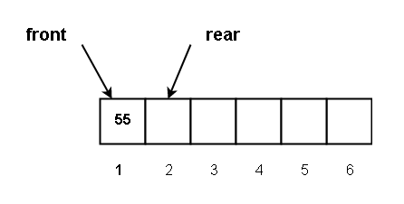
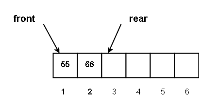
We inserted 55

Q [1] = 55, rear = 1 + 1 = 2, front = 1

This is shown in the following diagram.

We inserted another element 66, now the queue is

Q [2] = 66, rear = 2 + 1 = 3, front = 1

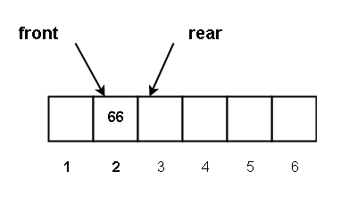
Now, let’s start deleting all the elements. Delete the first element 55. Then the queue status is as follows.

Rear = 3, front = 1 + 1 = 2 and Q [2] = 66

The element Q [1] = 55 is deleted.

Next, we delete the element Q [2] = 66. The status of the queue after deletion is shown below.

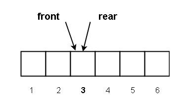
Now, front = 2 + 1 = 3, rear = 3 and since,

Front == rear

The queue is empty.

Queue Full Scenario

To insert into a queue, you need to check if the queue is full, so when the front == rear + 1, then the queue is full. Any attempt to insert a new element will result in queue overflow.

For example,

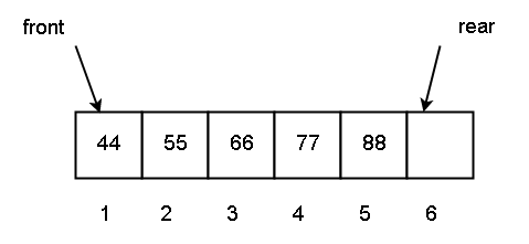
Current status of a queue is as follows

In the diagram above,

Q [1] = 44 and front = 1. Also Q [4] = 77 and rear = 5

Now we want to insert a new element 88 at Q [5].

The new status of the queue will be

Q [1] = 44 and front = 1, Q [5] = 88 and rear + 1 = 5 + 1 = 6

This is shown in the queue data structure diagram below.

Now finally, you will insert at Q [6] = 99. The status of the queue becomes

Q [1] = 44 and front = 1, Q [6] = 99 and rear + 1 = 6 + 1 = 7.

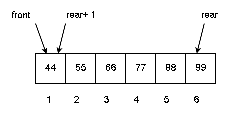
The rear value is greater than queue length. Then

rear + 1 = 7 mod 6 = 1

But,

front = rear + 1 = 1

Then the queue is full and we cannot insert more elements.

References

A.A.Puntambekar. 2009. Data Structures And Algorithms. Technical Publications.

E.Balaguruswamy. 2013. Data Structures Using C. McGraw Hill Education.

Thomas H. Cormen, Charles E. Leiserson, Ronald Rivest, Clifford Stein. 2009. Introduction to Algorithms. MIT Press.

C Program to find the biggest and smallest number and its location

Given an array of integer numbers, we sometimes need to find the largest and the smallest number from the array. This is not a problem if the array is already sorted in ascending or descending order.

This program finds the biggest and the smallest number from a given array of integers and also tell the index value (location) of those values.

We have used Dev-C++ 4.9.9.2 compiler installed on a windows 7 64-bit computer to run the program. You can do the same or use any other ANSI standard C compiler to run the program. The program is intended for beginners of C programming language.

Problem Definition

you are given an array of unsorted integers and you want to solve two problems.

1. Find biggest number
2. Find smallest number

To solve this problem very easily by

1. Assigning the first number from the array as the smallest number. You do not know yet, if this is the smallest number, we are just assuming it is.
2. Compare this smallest assumed value with other elements of the array and if you encounter another smaller value than the current smallest value, the new value becomes the smallest.
3. Then the process repeats itself, until search procedure is exhausted.

To find the biggest number do the same thing except the first value is assumed to be the largest value in the array.

Flowchart – Find Biggest and Smallest Number

Program Code

/* program to find the biggest and smallest number in an array of numbers. */

#include <stdio.h>
#include <stdlib.h>

#define SIZE 100 

main() {

/* declare variables array, smallest, biggest,
location_smallest,location_biggest,array_size,i*/

    int array_of_number[SIZE];
    int big_num,small_num,loc_small,loc_big;
    int i,n;

/* Get the size of the array input */

    printf("ENTER THE SIZE OF THE ARRAY:");
    scanf("%d",&n);

/* Get the Array elements */

    printf("GET THE ARRAY ELEMENTS:");

for(i=1;i<=n;i++) {

    scanf("%d",&array_of_number[i]); 

    }

/* Search for the biggest Number and it's location */

    big_num = array_of_number[1];

for(i=1;i<=n;i++) {

    if(big_num <= array_of_number[i]) {

        big_num = array_of_number[i];
        loc_big = i;
    }
}

printf("_________________________________________\n");

printf("The Biggest Number is %d at location = %d\n",big_num,loc_big);

printf("_________________________________________\n");

/* Find smallest number and it's location */

small_num = array_of_number[1];

for(i=1;i<=n;i++) { 

    if(small_num >= array_of_number[i]) {
        small_num = array_of_number[i];
        loc_small = i;
    }
}

printf("___________________________________________\n");

printf("The smallest Number is %d at location = %d\n",small_num,loc_small);

printf("___________________________________________\n");

    getch();
    return 0;
}


Output

ENTER THE SIZE OF THE ARRAY:5
GET THE ARRAY ELEMENTS:53
66
3
6
23
_________________________________________
The Biggest Number is 66 at location = 2
_________________________________________
_________________________________________
The smallest Number is 3 at location = 3
_________________________________________