Algorithms Notes – Concepts, Examples, MCQs & Exam-Ready Revision
Algorithms is a core subject in Computer Science and IT courses as well as competitive exams like GATE, UGC NET and university exams.
On this page, you will find structured resources to learn algorithm concepts, along with clear explanations, examples and exam-ready revision notes.
What will you learn
On this page you will find:
- Core algorithm concepts explained clearly and systematically
- Exam-oriented explanations supported with relevant examples
- MCQ-based practice posts to test your understanding
- Detailed articles along with exam-ready revision PDFs
This Page is for:
- Computer science and IT students
- GATE and other competitive exam aspirants
- University exam preparation
- Self learners
Topic Sections
Find Algorithms topics here.
(1) Algorithms Analysis Tools
(2) Sorting Algorithms
(3) Searching Algorithms
(4) Tree Based Algorithms
(5) Graph Based Algorithms
(6) Spanning Tree Algorithms
Algorithm Design Techniques
(A) Brute force Algorithms
(B) Divide and Conquer Algorithms
(C) Greedy Algorithms
(D) Dynamic Programming
(E) Backtracking
Selection Sort Algorithm
The selection sort algorithm is a sorting algorithm that selects the smallest element from an array of unsorted elements called a pass. In each pass, it selects an unsorted element from the array and compares it with the rest of the unsorted array.
If any element smaller than the current smallest is found, replace it with a new element. This process is repeated until there are no more small elements. The entire array is sorted in this way.
The steps performed in each pass is as follows.
- Given an array, $latex A[1\cdots n]&s=2$.
- Find the smallest element in the array, $latex A[1\cdots n]&s=2$.
- Replace with $latex A[1]&s=2$ with the resultant smallest element and repeat the process again for $latex a[2]&s=2$, and so on.
- Stop the search process when $latex n -1&s=2$ smallest elements are found, the last one is the largest in the array.
Selection-Sort Algorithm
Algorithm Selection-Sort(A)
{

for i = 1 to n-1
    i:= min

for j:= i +1 to n
    if A[j] < A[min]) then
        T: = A[min]
        A[min] := A[j]
        A[j] := T
}
Example of Selection Sort
In this example, we will sort 5 unsorted numbers.
\begin{aligned}
Array : (44, 7, 10, 77, 33)\\
Pass 1: (7, 44, 10, 77, 33)\\
Pass 2: (7, 10, 44, 77, 33)\\
Pass 3: (7, 10, 33, 77, 44)\\
Pass 3: (7, 10, 33, 77, 44)\\
Pass 4: (7, 10, 33, 44, 77)\\
The \hspace{1mm}sorted\hspace{1mm} array \hspace{1mm}is\hspace{1mm} (7, 10, 33, 44, 77)
\end{aligned}
Analysis of Selection Sort
The selection-sort algorithm has $latex 2 \hspace{2px} loops&s=2$ each time, the outer loop runs $latex n -1&s=2$ time and the inner loop runs as follows.
\begin{aligned}
&for \hspace{1mm} 1^{st}  \hspace{1mm}element  \hspace{1mm}of  \hspace{1mm}outer  \hspace{1mm}loop = n-1  \hspace{1mm}times\\
&for  \hspace{1mm}2^{nd}  \hspace{1mm}element  \hspace{1mm}of  \hspace{1mm}outer  \hspace{1mm}loop = n-2  \hspace{1mm}times, so \hspace{1mm} on\\
&for  \hspace{1mm} n-1^{th}  \hspace{1mm} element  \hspace{1mm}or  \hspace{1mm} outer  \hspace{1mm}loop = 1  \hspace{1mm}time
\end{aligned}
= ((n)(n-1))/2
= (5(5 - 1))/2
= 20/2
= 10 Let T(n) be the total running time of selection sort then,
\begin{aligned}
&T(n) = (4 + 3 + 2 + 1) \\
&= 10 \hspace{1mm}operations
\end{aligned}
The running time of the selection sort algorithm is then $latex \theta(n^2)&s=2$ for both best-case and worst-case. Even in best-case, we will run a comparison in sub-array in the same manner as worst-case. Thus, the running time is $latex \theta(n^2)&s=2$.
Hash Table
The hash table is perfect solution to store dictionary where each data is uniquely identified using a key. The dictionaries are implemented using arrays. The key are stored with the object itself and each data element has its own index value. Therefore, data is stored in the array as key-value pair.
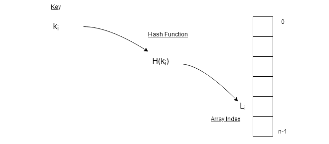
The hash table uses a hash function which is a mathematical function to compute a hash value $latex H(k)&s=2$ which is the index L of the data element in the array. The hash function uses key $latex k_{i}&s=2$ to compute $latex H(k_{i}) = L_{i}&s=2$.
The hash table allows three types of operations.
- Insertion of a new value.
- Deletion of an existing value.
- Search for a value in the array.
Direct Addressing Scheme
The hash table uses a numerical key or characters that are converted to numeric equivalent for computing the hash value $latex H_{k} = L&s=2$ where $latex L &s=2$ is the index of data element in the array.
Suppose $latex U&s=2$ is the universal set of all keys from where we use $latex k_{i}&s=2$ to map $latex L_{i}&s=2$ from an array of size $latex \lvert U \rvert &s=2$ It means every $latex k_{i}&s=2$ is mapped to every $latex L_{i} \in U&s=2$. Also, no two keys have same hash value.
This type assigning a unique value to each an every data element in array is called direct-addressing.
Example
In this example, our universe U = { all English letters } from where we get our keys $latex k_{i}&s=2$. The size of the array is $latex A[0: L-1]&s=2$ where $latex \lvert U \rvert&s=2$ is equal to $latex N&s=2$, the size of the array.
Each letter is a key is converted to a number equivalent to its position in the English alphabets. For example, A = 1, B = 2, and so on.
| Key | Hash Function | Hash Value |
| A | H(A) | 1 |
| B | H(B) | 2 |
| C | H(C) | 3 |
| D | H(D) | 4 |
| T | H(T) | 20 |
| V | H(V) | 22 |
| X | H(X) | 24 |
| Y | H(Y) | 25 |
| Z | H(Z) | 26 |
The direct-addressing is fine as long as the size of the data elements are small in number. Therefore, using a unique key for each an every element is impractical and difficult to maintain. We can use a small subset of keys $latex K&s=2$ from universal set of keys $latex U&s=2$ where $latex K < U&s=2$.
Another problem with direct addressing is computer memory, we cannot store all the values of array because memory size is limited.
Finally, the direct addressing requires you to use the whole array regardless of whether you want to store anything or not. The empty spaces are wasted.
Hash Function
If we are to use a small subset of keys such that $latex K = { k_{0}, k_{1} , . . . , k_{n-1}}&s=2$ maps all elements of array $latex A[0: N-1]&s=2$ where $latex N&s=1$ is the size of the array. Each array position has an index value $latex L_{i}&s=2$.
Hash function is a mathematical function such as a mod function which is a popular method of computing hash value. If range of the array is $latex A[0: N-1]&s=2$, for any key $latex k_{i}&s=2$,
\begin{aligned}
&H(k_{i}) = L_{i}\\
&H(k_{i}) = k_{i} \hspace{2 mm} MOD \hspace{2 mm} N
\end{aligned}
The MOD function takes a value as key and gives remainder as output. In this way, more than one key value or index will have same hash value.
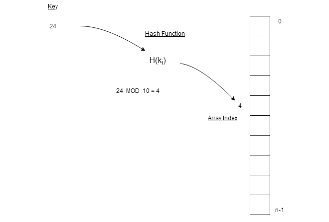
In the figure above, we have key $latex k = 24&s=2$ and $latex N = 10&s=2$ which is size of the array. A MOD operation on key $latex 24&s=2$ gives $latex 4&s=2$ which is the location of the data element in the array.
Similarly, if $latex key = 34&s=2$, then hash value is $latex 4&s=2$again. Therefore, we want a hash function which always gives same results for a key. The key values with same hash value are called synonyms.
Synonyms
We can treat hash value or index in an array as a bucket holding slots for each synonym. So, a bucket $latex b&s=2$ can be can have $latex s[0: m-1]&s=2$ slots. Such type of representation requires a two-dimensional array where a row indicates buckets with slots.
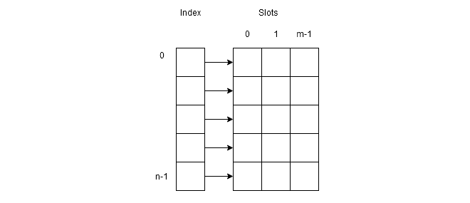
The figure above shows that the first column of the two dimensional array is buckets and other columns are slots.
Example
Let $latex K = { 20, 54, 32, 64, 21, 87, 42, 60, 77}&s=2$ be set of keys and size of array be $latex N = 10&s=2$. The hash function we are going to use is $latex H(k) = k MOD N&s=2$.
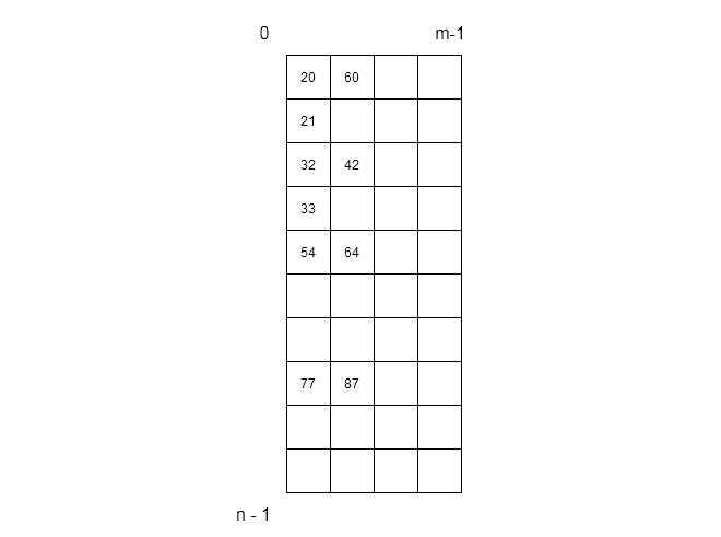
Each of the row in above figure has 3 slots per bucket to store values that have same hash values. for example,
\begin{aligned}
&77\hspace{2 mm} MOD \hspace{2 mm}10 = 7\\
&87\hspace{2 mm} MOD \hspace{2 mm} 10 = 7
\end{aligned}
Since, two slot have same value, it will cause problem during hash table operations – insertion, deletion and search.
Collision
When hash value is computed using hash function and if two keys $latex k_{i}&s=2$ and $latex k_{j}&s=2$ has same hash value then it cause a collision.
\begin{aligned}
&H(k_{i}) = H(k_{j})
\end{aligned}
Therefore, there are two important method of solving the problem of managing synonyms.
- Linear open addressing
- Chaining
In the future posts, we will talk about each of these methods in detail.
Fibonacci Search Algorithm
The Fibonacci search algorithm is another variant of binary search based on divide and conquer technique. The binary search as you may have learned earlier that split the array to be searched, exactly in the middle recursively to search for the key. Fibonacci search on the other hand is bit unusual and uses the Fibonacci sequence or numbers to make a decision tree and search the key.
Like binary search, the Fibonacci search also work on sorted array ( non-decreasing order).
The Fibonacci Sequence
Simply said the Fibonacci sequence is a set of numbers where any term $latex F_n&s=1$ is equal to the sum of previous two terms.
F_{n} = F_{n-1} + F_{n-2}If we try to generate first few terms of a Fibonacci sequence then we get the following numbers.
\begin{aligned}
&F_{0} = 0\\
&F_{1} = 1\\
&F_{2} = F_{1} + F_{0} = 1 + 0 = 1\\
&F_{3} = F_{2} + F_{1} = 1 + 1 = 2\\
&F_{4} = F_{3} + F_{2} = 2 + 1 = 3\\
&F_{5} = F_{4} + F_{3} = 3 + 2 = 5\\
&F_{6} = F_{5} + F_{4} = 5 + 3 = 8\\
&F_{7} = F_{6} + F_{5} = 8 + 5 = 13\\
&F_{8} = F_{7} + F_{6} = 13 + 8 = 21
\end{aligned}
Therefore, the Fibonacci sequence is as follows:
0, 1, 1, 2, 3, 5, 8, 13, 21, 34,...
Fibonacci Search
Algorithm Fibonacci_Search(A, n, key)
{
low:= 0
high:= n - 1
loc:= -1
flag:= 0
while(flag != 1 && low <= high)
{
// get the fibonacci f[m-1] < n
index:=get_fibonacci(n)
if ( key == A[index + low]) then
{
flag:= 1
loc:= index
break
}
else if ( key > A[index + low] ) then
{
//adjust the low
low:= low + index + 1
}
else
{
//adjust the high
high:= low + index - 1
}
//adjust the n
n:= high - low + 1
} // end of while
//return success or not
if ( flag = 1) then
{
return (loc + first + 1 )
}
else
{
return -1
}
} //end
Algorithm Fibonacci(n)
{
fibk2:= 0
fibk1:= 1
fibk:= 0
if ( n = 0 || n = 1) then
return 0
while ( fibk <n)
{
fibk:= fibk2 + fibk1
fibk2:= fibk1
fibk1:= fibk
}
return fibk2;
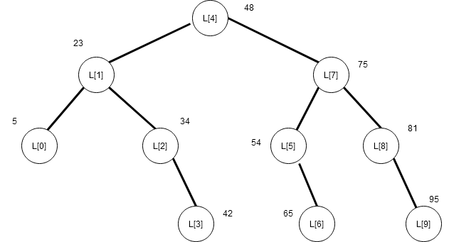
}How Fibonacci Search Works?
Fibonacci search uses the Fibonacci numbers to create a search tree. These are the steps taken during Fibonacci search.
Step 1:
The first step is to find a Fibonacci number that is greater than or equal to the size of the array in which we are searching for the key.
Suppose the size of the array is $latex n&s=1$ and fibonacci number is $latex F_{k}&s=2$.
We must find a $latex F_{k}&s=2$ such that
$latex F_{k} \geq n&s=2$
if $latex n = 10&s=2$ then we must find a $latex F_{k} \geq n&s=2$.
The Fibonacci sequence is
\begin{aligned}0, 1, 1, 2, 3, 5, 8, 13, ...\end{aligned}Therefore, $latex F_{k} = 13&s=2$ because $latex 13 \geq 10&s=2$.
Step 2:
The next step is to compare the key with the element at Fibonacci number $latex F_{k-1}&s=2$.
We know that $latex F_{k} = 13&s=2$ because $latex 13 \geq 10&s=2$. We must find the $latex F_{k-1} &s=2$.
Once again we look at the Fibonacci sequence is
\begin{aligned} 0, 1, 1, 2, 3, 5, 8, 13, ...\end{aligned}Since,
$latex F_{k} = F_{k-1} + F_{k-2}&s=2$
$latex 13 = 8 + 5&s=2$
$latex F_{k-1} = 8 &s=2$
Step 3:
If the key and array element at $latex F_{k-1}&s=2$ are equal then the key is at $latex F_{k-1} + 1&s=2$.
For example, we are searching within an array of 10 elements.
\begin{aligned}&10\hspace{3ex}34\hspace{3ex}39\hspace{3ex}45\hspace{3ex}53\hspace{3ex}58\hspace{3ex}66\hspace{3ex}75\hspace{3ex}83\hspace{3ex}88\\ \\
&A[0]\hspace{1ex} A[1]  \hspace{1ex} A[2]  \hspace{1ex} A[3] \hspace{1ex}  A[4] \hspace{1ex}  A[5]  \hspace{1ex}A [6]  \hspace{1ex} A[7] \hspace{1ex}  A[8] \hspace{1ex}  A[9]\end{aligned}
$latex n = 10&s=2$ and $latex F_{k} = 13&s=2$
Let $latex key = 83&s=2$ and $latex F_{k-1} = 8&s=2$
Therefore, key == A[8] is true.
Then the key is found at $latex F_{k-1} + 1&s=2$ which is $latex 8 + 1 = 9^{th}&s=2$ position.
Step 4:
If the key is less than array element at $latex F_{k-1}&s=2$, then search the left sub-tree to $latex F_{k-1}&s=2$.
For example, we are searching within an array of 10 elements.
\begin{aligned}
&10\hspace{3ex}34\hspace{3ex}39\hspace{3ex}45\hspace{3ex}53\hspace{3ex}58\hspace{3ex}66\hspace{3ex}75\hspace{3ex}83\hspace{3ex}88\\ \\
&A[0] \hspace{1ex}    A[1]\hspace{1ex}     A[2]  \hspace{1ex}   A[3]  \hspace{1ex}   A[4]\hspace{1ex}     A[5] \hspace{1ex} A[6] \hspace{1ex}    A[7]\hspace{1ex}     A[8]    \hspace{1ex} A[9]\end{aligned}
$latex n = 10&s=2$ and $latex F_{k} = 13&s=2$
Let $latex key = 39&s=2$ and $latex F_{k-1} = 8&s=2$
If key < A[8] is true,
Then search A[0:7] = { 10, 34, 39, 45, 53, 58, 66, 75 }
Step 5:
If the given key is greater than the array element at $latex F_{k-1}&s=2$, then search the right sub-tree to $latex F_{k-1}&s=2$.
\begin{aligned} &10\hspace{3ex}34\hspace{3ex}39\hspace{3ex}45\hspace{3ex}53\hspace{3ex}58\hspace{3ex}66\hspace{3ex}75\hspace{3ex}83\hspace{3ex}88\\\\
&A[0]\hspace{1ex} A[1] \hspace{1ex}  A[2] \hspace{1ex}  A[3]  \hspace{1ex} A[4] \hspace{1ex}  A[5]  \hspace{1ex} A[6]   \hspace{1ex}  A[7]  \hspace{1ex} A[8] \hspace{1ex}  A[9]\end{aligned}
$latex n = 10&s=2$ and $latex F_{k} = 13&s=2$
Let $latex key = 83&s=2$ and $latex F_{k-1} = 8&s=2$
If key > A[8] is true,
Then search A[9:9] = { 88 }
Step 6:
If the key is not found, repeat the step step 1 to step 5 as long as $latex F_{k-1} = 0&s=2$, that is, Fibonacci number >= n. After each iteration the size of array $latex n&s=1$ is reduced.
Fibonacci Search Example
In this example, we will take a sorted array and find the search key with the array using Fibonacci search technique. Each iteration will show you the state of lower index, higher index and current value of size n, and Fibonacci number used to locate the key.
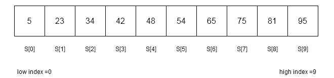
Consider the following sorted (non-decreasing) array with 10 elements.
Iteration 1
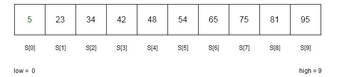
There are 10 elements in the above sorted array S. Therefore,
low = 0
n = 10
high = n-1 = 9
index = get_fibonacci(n) = 8 //because F_{k} = 13
loc = -1 //currect location of the key is outside array
flag = 0 //check whether key is found or not , flag = 1 indicates it is found
key = 65 // we are trying to find 65 in the array
is key == S[ index + low] ?
65 == 81 => NO
is key > S [ index + low] ?
65 > 81 => NO
is key < S[ index + low ] ?
65 < 81 =>YES
high = low + index - 1 // adjust the higher index and keep the low = 0
high = 0 + 8 - 1 = 7
n = high - low + 1 // adjust the size of the array
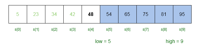
n = 7 - 0 + 1 = 8Iteration 2
![Figure 2- key is less than S[8]. We must search left sub-tree. The array size n is adjusted to 8 elements.](https://notesformsc.org/wp-content/uploads/2020/12/Figure2-Fibonacci-Search-Array.png)
There are 8 elements in the above sorted array S. Therefore,
low = 0
n = 8
high = 7
index = get_fibonacci(n) =  5    //because previous F_{k} = 8
loc = -1                         //currect location of the key is outside array
flag = 0                         //check whether key is found or not , flag = 1 indicates it is found
key = 65                         // we are trying to find 65 in the array
is key == S[ index + low] ?
65 == 54 => NO
is key > S [ index + low] ?
65 > 54 => YES                  // key is higher than the array element S[5], move to right sub=-tree

low = low + index + 1           // adjust the lower index and keep the high = 7
low = 0 + 5 + 1 = 6
n = high - low + 1              // adjust the size of the array
n = 7 - 6 + 1 = 2
Iteration 3
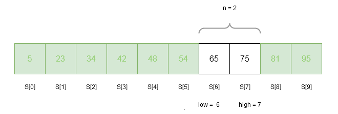
There are 2 elements in the above sorted array S. Therefore,
low = 6
n = 2
high = 7
index = get_fibonacci(n) =  1    //because previous F_{k} = 5
loc = -1                         //currect location of the key is outside array
flag = 0                         //check whether key is found or not, flag = 1 indicates it is found
key = 65                         // we are trying to find 65 in the array
is key == S[ index + low] ?
65 == 75 => NO
is key > S [ index + low] ?      // key is higher than the array element S[1], move to right sub=-tree
65 > 75 => NO
is key < S[ index + low ] ?      // key is higher than the array element S[1], move to left sub=-tree
65 < 81 =>YES

high = low + index - 1           // adjust the lower index and keep the high = 7
high =  6 + 1 - 1 = 6
n = high - low + 1              // adjust the size of the array
n = 6 - 6 + 1 = 1
Iteration 4
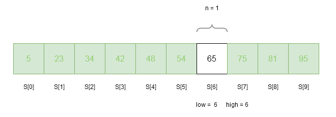
Only 1 element remained in the array, still we must go through the iteration.
low = 6
n = 1
high = 6
index = get_fibonacci(n) =  0    // because when n = 0 or n = 1, simply return 0.
loc = -1                         //currect location of the key is outside array
flag = 0                         //check whether key is found or not , flag = 1 indicates it is found
key = 65                         // we are trying to find 65 in the array
is key == S[ index + low] ?      // A[ 6 + 0] = S[6] = 65
65 == 65 => YES
flag = 1
Key is found !
Time Complexity of Fibonacci Search
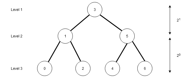
Here is the Fibonacci search decision tree for $latex n=10&s=2$.
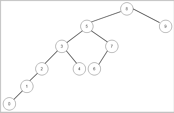
The Fibonacci search also perform like binary search on a sorted array; therefore, the time complexity is in worst case is $latex O( log\hspace{1ex} n)&s=2$.
We can clearly note a few things from the above decision tree.
If the difference in index of grandparents and parent of a node is $latex F_{k}&s=2$ then
- The left sub-tree is of order $latex F_{k-1}&s=2$.
- The left sub-tree is of order $latex F_{k-2}&s=2$.
- This is true for every sub-tree.
- The difference between parent and both children is the same.
- The leftmost path represents a Fibonacci sequence that starts with 0, 1, 2, 3, … .
C++ Implementation Of Fibonacci Search Algorithm
#include <iostream.h>
#include <stdio.h>
#include <conio.h>
int get_fib(int);
int main()
{
  int S[10]= { 5, 23, 34, 42, 48, 54, 65, 75, 81, 95 };
  int n,key, index, low, high, loc, flag;
  n = 10;
  low = 0;
  int location = -1;
  high = n-1;
  flag = 0;  //Read the key
  cout << "Enter Key To Search:";
  cin >> key;
  index = 0;
  while ( flag != 1 && low <= high)
  {
     index = get_fib(n);
     if ( key == S[index + low])
     {
	location = low + index;
	flag = 1;
	break;
     }
     else if( key > S[index + low])
     {
	low = low + index + 1;
     }
     else
     {
	high = low + index -1;
     }
     n = high - low + 1;
  }
     if ( flag == 1)
     {
	cout << "Element Found at Index =" << location << endl;
     }

  getch();
  return 0;
  }

int get_fib(int n)
{
  int fibk = 0;
  int fibk2 = 0;
  int fibk1 = 1;
  if( n == 0 || n == 1)
  {
     return 0;
  }
      while(fibk < n)
      {
	 fibk = fibk1 + fibk2;
	 fibk2 = fibk1;
	 fibk1 = fibk;
      }
      return fibk2;
 }
Input
Enter Key To Search:65Output
Element Found at Index = 6In the next post, we shall discuss about searching though Hash Table.
Binary Search Algorithm
The binary search algorithm is very popular search algorithm. It is also known as half-interval search or uniform binary search as it split the array of data into two equal parts recursively until a solution is found. The array in binary search must be sorted.
Binary search employ an algorithm design technique known as divide and conquer. In this technique, a given problem is divided into smaller sub-problems and this is done until no more sub-division is possible.
Then solution to the smallest problem is found and all solutions are combined to get the overall solution to the problem. The divide and conquer technique is not limited to binary search; therefore, we shall discuss this separately in another article.
Binary Search Algorithm
Algorithm Binary Search (S, n , key)
{
   low := 0
   high = n - 1
   while (low <= high)
   {
      //compute the mid value
      mid = low + (high - low)/2
      if (key < S[mid]) then
          high := mid - 1
      else if ( key > S[mid]) then
          low := mid + 1
      else
          return mid
   }
}
The elements of binary search are as follows.
$latex S[ ]&s=2$ – The sorted array with data.
$latex n&s=2$ – It is the number of elements in the array.
$latex key&s=2$ – The search key to be found.
Mid Value
The mid value is most important in binary search as it split the array in to two parts. Then the sub-array is split in the similar way based on divide and conquer technique. The mid is an index of the element in the middle of the array.
mid = low + (high - low)/2How Binary Search Works?
The binary search works on a sorted array. Suppose we have an array with elements in non-decreasing order. To search for a given key, binary search will compute the mid value and thus break the array into equal halves. The key is compared with array element with index value as mid.
Suppose our $latex key&s=2$ is $latex 65&s=2$, then $latex mid&s=2$ is calculated as follows.
mid = 0 + ( 9 - 0 ) / 2 = 0 + 4 = 4

//S[4] = 48
//key > S[mid] ( 65 > 48  )
//low = mid + 1

low = 4 + 1 = 5

//low = 5 and high = 9
Now we will consider the upper half of the array for searching with $latex low = 5&s=2$ and $latex high = 9&s=2$.
We now have to compute a new mid value in the upper half of the array to search for the key.
mid = 5 + ( 9 - 5 )/2
mid = 5 + 4/2
mid = 5 + 2
mid = 7

//S[7] = 75
//key < S[mid] (65 < 75 )
//high = mid - 1

high = 7 - 1
high = 6

//now, low = 5 and high = 6
We will compute the new mid value with $latex low = 5&s=2$ and $latex high = 6&s=2$.
![Figure 3- The old mid is 75 and low = 5 with new high = 6. Our search is limited to S[5] and S[6] only.](https://notesformsc.org/wp-content/uploads/2020/12/Figure3-BinarySearcArray.png)
We only have two element to search for the key. The $latex mid&s=2$ is calculated using $latex high = 6&s=2$ and $latex low = 5&s=2$.
mid = 5 + ( 6 - 5 )/2
mid = 5 + 0
mid = 5

//S[5] = 54
//key > S[mid] ( 65 > 54 )
//low = mid + 1

low = 5 + 1
low = 6

//low = 6 and high = 6
The high and low are equal which will be last iteration of while loop in the binary search algorithm. However, $latex mid&s=2$ is still calculated for the last iteration.
mid = 6 + ( 6 - 6 )/2
mid = 6 + 0
mid = 6

//key == S[mid] ( 65 == 65 )
//mid is returned 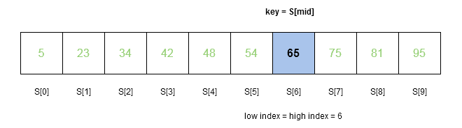
Time Complexity Of Binary Search
How much time binary search take on average to search for an element in the array ? Before we try to answer that question, let us understand the decision tree for binary search.
A decision tree is the pattern that the binary search follows to get to the element. Suppose that each of the node in binary search has two child including the root. Then the total number of nodes in the decision tree is given by the equation.
\begin{aligned}
&N <= 2^L - 1\\
&N + 1 <= 2^L\\

&Where \\
&N \hspace{1mm} is \hspace{1mm}total \hspace{1mm} number \hspace{1mm} of \hspace{1mm} nodes\hspace{1mm}  in \hspace{1mm} the\hspace{1mm}  decision\hspace{1mm} tree.\\
&L \hspace{1mm} is \hspace{1mm} the \hspace{1mm} number\hspace{1mm} of \hspace{1mm}levels\hspace{1mm}  in \hspace{1mm} the\hspace{1mm} decision\hspace{1mm} tree.
\end{aligned}
The decision tree above is from an array of size $latex 7&s=2$ where $latex root = 3&s=2$ is the mid value. If we compute other mid values we get the above decision tree. The difference between parent and child is $latex 2^x&s=2$ where $latex x = 0, 1, 2 ,\cdots&s=2$.
Relationship between Nodes and Elements of Sorted Array
In the above decision tree, we have number of elements that match with the tree. Each of the node in the decision tree has exactly 2 child. But this is not possible all the time because number of elements $latex (n)&s=2$ of an array for binary search can be different.
Therefore,
\begin{aligned}
&N + 1 >= n + 1\\
&where \\
&N + 1  \hspace{1mm}is \hspace{1mm}the\hspace{1mm} number\hspace{1mm} of\hspace{1mm} nodes\hspace{1mm} in the\hspace{1mm} tree\\
&n + 1\hspace{1mm} is \hspace{1mm}the \hspace{1mm}number \hspace{1mm}of \hspace{1mm}elements\hspace{1mm} in \hspace{1mm}the \hspace{1mm}array
\end{aligned}
Using the above information we can say that
2^L >= N + 1 >= n + 1
Taking log of equation will give us, $latex log (n + 1)&s=2$. Therefore, the time complexity of binary search in average and worst case is given as $latex O(log \hspace{1ex} n)&s=2$.
C++ Implementation of Binary Search
#include <iostream.h>
#include <stdio.h>
#include <conio.h>
int main()
{
   int S[10] = { 6, 23, 34, 42, 48, 54, 65, 75, 81, 95};
   int key,low,high;
   int mid= 0;
   //Read key value
   cout <<"Enter your key:" ;
   cin >> key;
   low = 0;
   high = 9;
   //Binary search
   while(low <= high)
   {

      mid = low + (high - low)/2;

      if (key < S[mid])
      {
	high = mid - 1;
      }
      else if ( key > S[mid])
      {
	  low = mid + 1;
      }
      else
      {

      cout <<"Key found at " << mid << ": " << S[mid]<<endl;
      return mid;
      }
   }
 }
Input:
Enter your key: 65Output:
Key found at 6: 65In the next article, we will discuss another variant of binary search called the interpolation search.
Interpolation Search Algorithm
The interpolation is an advanced version of binary search algorithm. It performs better than the binary search algorithm for large data sets.
Remember how we look for a word in the dictionary. If you want to search for word “Cat” immediately we open that part of the dictionary because we have an idea about where to look for that word. A word that starts with letter ‘T’ then you would jump to that location in the dictionary which contains all words that start from letter ‘T’. The interpolation search is inspired by this idea of finding the key based on its probed position from the beginning of the array.
Like binary search, the interpolation search also need a sorted array.
Interpolation Search
Algorithm interpolation_search(S, n, Key)
{
    low := 0
    high := n - 1
    mid := 0

    while ((S[high] != S[low]) && (key >= S[low]) && (key <= S[high])) {
        mid = low + ((key - S[low]) * (high - low) / (S[high] - S[low]));

        if (S[mid] < key)
            low = mid + 1;
        else if (key < S[mid])
            high = mid - 1;
        else
            return mid;
    }

    if (key = S[low])
        return low
    else
        return -1
}
In the above pseudo code we have following
S[ ] – It is the array with n elements.
n – It is the number of elements in the given array.
Key – it is the search key we are trying to locate within the array.
low – lowest index which start at 0
high – highest index which is n-1 if low starts at 0.
mid – middle value of the array.
How Interpolation Search Works?
Suppose you have to search a number between 0 to 99. You are given an array of size 10 to search and all number are equally distributed. Consider the image below.
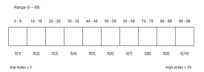
Each position has a separate range of number possible because the array must be sorted. So, in first position we can have any number from 0-9 and second position we can have a number between 20-29 and so on.
The numbers may or may not be equally distributed. Suppose if the numbers are equally distributed as per the figure below.
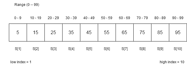
The interpolation search will use the following equation to probe the position of middle (mid) element. If right index is found return the index or continue the probe.
mid = low + (x - S[low]) * (high - low)/(S[high] - S[low])Suppose we want to search for x = 35 from the array. Then using the above equation, we get,
mid = 1 + ( 35 - 5 ) * ( 10 - 1 ) / ( 95 - 5 )
= 1 + 30 * 9 / 90
= 1 + 270/ 90
= 1 + 3 => 3
Therefore, S[4] = 35
We were directly able to probe the correct position of the search key 35.
Let us consider another situation where array is not distributed equally, however, the array is sorted in non-decreasing order. See the image below.
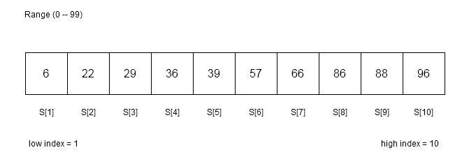
In this array, we must search for key = 86 using interpolation search technique. The algorithm determine if the search key falls within the range S[low] and S[high], otherwise it will report false and terminate.
The next step is to compute the mid value using equation of mid.
mid = 1 + (86 - 6 ) * ( 10 - 1 ) / ( 96 - 6 )
mid = 1 + ( 80 * 9 ) / 90
mid = 1 + 720/90
mid = 1 + 8 = 9
S[9] = 88
We did not get the right value in the first iteration; therefore, interpolation search will run another iteration to find the search key = 86.
If key < S[mid] then
high = mid - 1
Then run the interpolation search again.
low = 1
high = 9 - 1 = 8
S[1] = 6
S[8] = 86
x = 86
mid = 1 + ( 86 - 6 ) * (8 - 1)/ (86 - 6)
mid = 1 + 80 * 7 / 80
mid = 1 + 7
mid = 8
S[8] = 86
Key is found !
Binary Search and Interpolation Search
By probing the correct position or even closer to the key in an array, the interpolation search takes full advantage of the sorted array where binary search will take more steps by splitting the array into half the size repeatedly. In smaller searches the binary search may be faster than interpolation search, but if you have an extremely big data to search interpolation search algorithm will take less time.
In the above example, to search for key = 86, the interpolation search took 2 steps to complete. The above computation will give you an idea that the binary search is not good when compared with interpolation search while working on a large data set.
Time Complexity
On average the interpolation search perform better than binary search.The time complexity of binary search in average case and worst case scenario is $latex O( log \hspace{1ex} n)&s=2$.
The interpolation search on average case has $latex O(log (log \hspace{1ex} n))&s=2$ assuming that the array is evenly distributed. If the array is increasing exponentially then the worst case happens. Then we must compare the search key to each element of the array. This will give a time complexity of $latex O(n)&s=2$.
C++ Implementation of Interpolation Search
#include <iostream.h>
#include <stdio.h>
#include <conio.h>
int main()
{
   int S[10] = { 6, 22, 29, 34, 43, 57,66, 86, 88, 96};
   int key,low,high;
   int mid= 0;
   //Read key value
   cout <<"Enter your key:" ;
   cin >> key;
   low = 0;
   high = 9;
   //Interpolation search
   while((S[low] != S[high]) && (key >= S[low]) && ( key <= S[high]))
   {

      mid = low + ((key - S[low]) * (high - low)/(S[high] - S[low]));

      if (S[mid] < key)
      {
	low = mid + 1;
      }
      else if ( key < S[mid])
      {
	  high = mid - 1;
      }
      else
      {

      cout <<"Key found at " << mid << ": " << S[mid]<<endl;
      return mid;
      }
   }

   if ( key == S[low])
   {
      return low;
   }
   else
   {
      return -1;

   }

   }
Input
Enter your key:22Output
Key found at 1: 22Transpose Sequential Search
Earlier you learned about linear search which search for a key from a given array. The search is affected by whether the array is ordered or unordered. The performance get better if the key is found at the beginning of the array. The transpose sequential search does that for repeated searches. It is also known as self-organizing linear search.
With each time you search for a key in the array, the transpose sequential search will shift the key at the beginning of the array. Therefore, next time you search for the same key you will find it in less time.
Transpose Sequential Search Algorithm
//Algorithm : Transpose Sequential Search
Algorithm Transpose_Sequential_Search(S, n, K)
{
     i := 0
     while (i < n and K != S[i]) do
     {
          i := i + 1         // move through the array as long as K is not matching any element
     }
     if K = S[i] then
     {
          print ("Key found !")
          swap( S[i], S[i-1])
     }
     else
     {
          print ("Key not found !")
     }
}
In the algorithms above,
$latex K&s=2$ – It is the search key which we are trying to locate in the array.
$latex S [0: n-1]&s=2$ – It is the array of numbers.
$latex n&s=2$- it is the number of elements in the array.
Example #1
Suppose there is an array $latex S&s=2$ of $latex 10&s=2$ numbers and we want to search for a key $latex K&s=2$. We will do the usual search, but repeat our search several times for the same key $latex K&s=2$. This will show us the use of transpose sequential search in repeated searches.
Let \hspace{1mm}S[0: 9] = \{ 42, 54, 10, 59, 32, 11, 77, 21, 99, 66 \} \hspace{1mm} and \hspace{1mm} search \hspace{1mm} key \hspace{1mm} be \hspace{1mm} K = 99.We will do repeated search for $latex K&s=2$ in following way.
99, 10, 99, 32, 99
In between our searches, we are trying to search other numbers also, so that it look natural. With each search attempt the original array will change in following way.
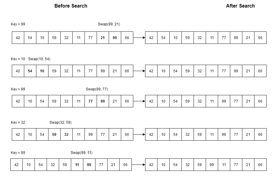
Each of the search will swap the search key with its previous element, if we are searching for $latex 99&s=2$ , first it gets found and then it is swapped with previous element $latex 21&s=2$ initially. With each subsequent search the position of $latex 99&s=2$ goes to the beginning of the array.
Time Complexity of Transpose Sequential Search
If the search key $latex K&s=2$ is at the end of the array then it is worst case scenario and time taken is $latex O(n)&s=2$. Each search attempt improves the position and the search is done in constant time $latex O(1)&s=2$.
C++ Implementation of Transpose Sequential Search
PROGRAM : TRANSPOSE SEQUENTIAL SEARCH
#include <iostream.h>
#include <stdio.h>
int main()
{
//Declare all variables and the array
 int S[] = { 42, 54, 10, 59, 32, 11, 77, 21, 99, 66 };
 int K;
 int temp = 0;
 int n = 10;
 int i = 0;
 // Read the input value
 cout << "Input the value of K: ";
 cin >> K;
 while (i < n && K != S[i])
 {
    i = i + 1;           //Move through the array
 }
 if(K == S[i])
 {
    cout << "Key Found!" << endl;
    //swap
    temp = S[i];
    S[i] = S[i-1];
    S[i-1] = temp;
    cout << S[i-1];
 }
 else
 {
    cout << "Item not found" << endl;
 }

 return 0;
}
Input:
Input the value of K: 99Output :
Key Found!
99
In the next article, you will learn about some other forms of linear search algorithms.
Linear Search Algorithms
The linear search is the simplest search where we try to find an element K from the list L. We have to compare K with each and every item in the list. The search is affected when the list if sorted or unsorted.
Linear Search
Suppose we want to find search key $latex K&s=2$ from array $latex S&s=2$ with elements
\{ s_1, s_2, s_3, s_4,\cdots,s_n \}There is two possible situations.
- The array $latex S&s=2$ is ordered from lowest to highest.
- The array $latex S&s=2$ is unordered.
If the array is sorted then the search is called an ordered linear search. If a search is performed on unordered array then it is called an unordered linear search.
Unordered Linear Search
Algorithm Ordered_Linear_Search ( S, n, K)
{
// S[0: n-1] is the array with n sorted elements
// n is the total number of elements in the array
// K is the key we are trying to find in the array S

i : = 0
while (i < n and K > S[i]) do   //keep moving through the elements
{
      i := i + 1
}
if K = S[i] then
      print("Key found!")
      return(i) // return the index of the element found
else
      print("Key not found!")
}
In the above algorithm, we have following:
$latex S[0: n-1]&s=2$ – An array with n elements that is sorted already.
$latex n&s=2$ – It is the number of elements in the array. The array starts with index $latex 0&s=2$ and that last element has an index of $latex n-1&s=2$.
$latex K&s=2$ – It is the value we are searching within the array. If found then algorithm return the location index of $latex K&s=2$ else it will simply print “Not found”. $latex K&s=2$ is called the search key.
Example #1
Suppose we have an array of numbers,
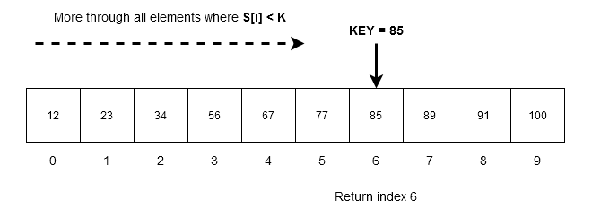
S[0: 9] = \{ 12, 23, 34, 56, 67, 77, 85, 89, 91, 100 \}We want to search for $latex K = 85&s=2$ in the array. The algorithm goes through each item in the array as long as
- $latex K&s=2$ is greater than element $latex S[i]&s=2$, that is, $latex K&s=2$ is greater than any element in the array keep moving.
- When $latex K&s=2$ is equal to any element $latex K[i]&s=2$ ,that is, $latex K = S[i]&s=2$. We have found the element successfully and return the index value.
In the above example, $latex 12, 23, 34, 56, 67, 77&s=2$ are less than $latex K = 85&s=2$; therefore, search algorithm will skip all of these elements and stop at $latex K = S[i] = 85&s=2$ which is true. The index $latex i = 6&s=2$ is returned.
Note that the ordered linear search will not continue anymore and terminate successfully.
Time Complexity of Ordered Linear Search
Since the array is ordered, it is easy to compute the time complexity. If the search key is at the beginning which is the best case, it takes $latex \O(1{})&s=2$ constant time to find the element.
What if the element is not available ? The algorithm goes through each and every element in the array. If array has n element then the complexity is $latex \O(n{})&s=2$ which is the worst case.
C++ Implementation Of Ordered Linear Search
//PROGRAM: ORDERED LINEAR SEARCH
#include <iostream.h>
#include <stdio.h>
int main()
{
//Declare all variables and the array
 int S[] = {12,23,34,56,67,77,85,89,91,100};
 int K;
 int n = 10;
 int i = 0;
 // Read the input value
 cout << "Input the value of K: ";
 cin >> K;
 while (i < n && K > S[i])
 {
    i = i + 1;           //Move through the array
 }
 if(K == S[i])           //Check if the key is equal to any element in the array
 {
    cout << "Key Found!" << endl;
    cout << "Location = " << i << endl;
 }
 else
 {
    cout << "Item not found" << endl;
 }

 return 0;
}
Program Input :
Input the value of K: 85Program Output:
Key Found!
Location = 6
Unordered Linear Search
The unordered linear search is where the array has unordered elements. If we want to search for the key, then we must go through all elements.
Algorithm Unordered_Linear_Search ( S, n, K)
{
// S[0: n-1] is the array with n sorted elements
// n is the total number of elements in the array
// K is the key we are trying to find in the array S

i : = 0
while (i < n and K != S[i]) do   //keep moving through the elements until a match is found
{
      i := i + 1
}
if K = S[i] then
      print("Key found!")
      return(i) // return the index of the element found
else
      print("Key not found!")
}
The above algorithms is similar to ordered linear search, however it does not search in ascending order or descending order. The array may contain the key value at any location.
Example #2
Suppose an unordered array contain following elements,
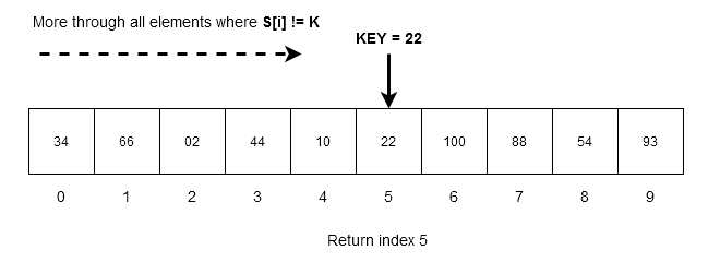
S[0: 9] = \{ 34, 66, 02, 44, 10,100, 22, 88, 54, 93 \}We want to search for $latex K = 22&s=2$ in the array. The algorithm goes through each item in the array as long as elements are not equal to the key.
Time Complexity of Unordered Linear Search
The time complexity is very much similar to ordered linear search. If you locate the element at the beginning of the search then the complexity is $latex O(1)&s=2$ and worst case it is $latex O(n)&s=2$.
But, think about search on average the ordered array will stop searching as soon as the right element is found and unordered array has to go through all elements because the key could be scattered anywhere.Therefore, ordered linear search perform better on average.
C++ Implementation Of Unordered Linear Search
#include <iostream.h>
#include <stdio.h>
int main()
{
//Declare all variables and the array
 int S[] = {34, 66, 2, 44, 10, 22, 100, 88, 54, 93 };
 int K;
 int n = 10;
 int i = 0;
 // Read the input value
 cout << "Input the value of K: ";
 cin >> K;
 while (i < n && K != S[i])
 {
    i = i + 1;           //Move through the array

 if(K == S[i])
 {
    cout << "Key Found!" << endl;
    cout << "Location = " << i << endl;
 }
 else
 {
    cout << "Item not found" << endl;
 }

 return 0;
}
Program Input:
Input the value of K: 22Program Output:
Key Found!
Location = 5
In the next article, you will learn about other linear search algorithms.
Algorithms – Search Techniques Overview
Searching for information is a basic task that we all do. We search for an item in a grocery list, or look for a telephone number from the telephone directory. A common and popular example of searching is Google search where we search for links to web sites such as Notesformsc, or look for specific images, text and so on.
The searching techniques differ depending on the type of data where we are performing the search. Your goal is to get the information as fast as possible and this is due to enormous repository of information available today.
Searching And Data Structures
Searching techniques have very close relationship with data structures. The data structure influence the choice of search techniques. Therefore, we classify data structures into following classes.
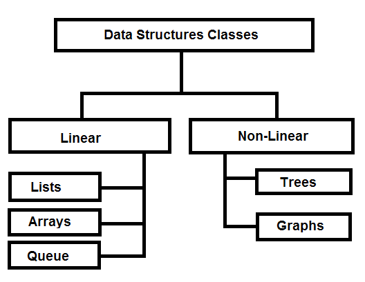
Linear Structures
When the data structure is in the form of lists than we can use following type of searches algorithms.
- Linear search or sequential search
- Transpose sequential search
- Interpolation search
- Binary search
- Fibonacci search
Non-Linear Structures
The non-linear data structures are trees like binary search trees, AVL trees, etc or you have graphs to search. There are hash tables which also introduce some interesting search techniques. A tree search can employ recursive or iterative search within the tree.
For graph based data structures, the following algorithms are very popular.
- Breadth first search
- Depth first search
Files And Databases
Database searches are done on large volume of data.The data is stored in files and indexed with key/value pair that assist in quick searches. These kind of searches are called indexed sequential searches.
In this section, we will be discussing about various search algorithms and their performances.
Algorithm Time Complexity
Given a piece of code, how to determine the complexities without much effort? Each piece of code has a time complexity associated with it which you need to learn. Next time, you see any complex code break it into individual pieces and count the time complexity.
Before you begin, learn the basics of algorithm performance and its complexity.
An algorithm has following types of code and we are going to learn time complexity for each one of them.
- Statements
- If-Then-else
- Loops
- Nested loops
- Functions
- Statements with functions.
Statements
Each of the statement in an algorithm takes a constant time to execute. If the algorithm procedure has N statements.
Then,
statement 1;

statement 2;

statement 3;

statement n
\begin{aligned}
&Constant \hspace{1mm}time = \mathcal{O}(1)\\ \\
&Total\hspace{1mm} running \hspace{1mm}time = \mathcal{O}(1) + \mathcal{O}(1) + \dots+ \mathcal{O}(1)\\ \\
\end{aligned}Sum of all the constant times is also a constant.
Therefore,
The Total running time is also constant $latex \mathcal{O}(1)&s=1$.
If-Then-Else
For the if-then-else block, only one block gets executed, based on the condition. But the run time for the block may be different from other blocks in the if-then-else statement.
if (condition) then
{

    block 1;

}
else
{

    block2;

}
Therefore,
\begin{aligned}
Total \hspace{1mm}runtime = Max(time(block 1), time(block2));
\end{aligned}
For Example,
Total\hspace{1mm} runtime = Max(\mathcal{O}(1), \mathcal{O}(n))Depending on the condition the total runtime of if-then-else block could be
\mathcal{O}(1) \hspace{1mm}or\hspace{1mm} \mathcal{O}(n)Loops
The loop runs for N time for any given N value. The statements inside the loop also get repeated for N times.
for j = 1 to N do {

    statements;

}
The loop runs for N time and each of the statements inside the loop takes $latex \mathcal{O}(1)&s=2$. Then the total runtime is given below.
\begin{aligned}
&Total \hspace{1mm}runtime = N * \mathcal{O}(1)\\
&=  \mathcal{O}(N)
\end{aligned}
Nested Loop
The nested loop is not different than the single loop statement. Now that there are two loops their running time get multiplied.
for i = 1 to N do
{

    for j = 1 to M do
    {

        Statements;

    }
}
Suppose the outer loop runs $latex N&s=2$ times and an inner loop has a complexity of $latex \mathcal{O}(M)&s=2$.
Total \hspace{1mm}Time\hspace{1mm} Complexity = \mathcal{O}(N * M)Let us say that the inner also runs for N times, the total complexity is given by
= \mathcal{O}(N^2)Functions
Functions are blocks themselves and contain many other statements. The total time of a function depends on these statements.
Suppose a function $latex f(N)&s=2$ takes $latex \mathcal{O}(1)&s=2$ and there is another function $latex g(N)&s=2$ that has a loop. Then,
Total \hspace{1mm}Time\hspace{1mm} Complexity \hspace{1mm}of \hspace{1mm}g(N) = \mathcal{O}(N)because of the loop.
Statements with Function
A loop statement can be inside of a function, but it is also possible that a function is inside of a loop.
for j=1 to N do {

    g(N);

}
Since, we already know that the running time of the function $latex g(N)&s=2$ is $latex \mathcal{O}(N)&s=2$.
\begin{aligned}
&Total \hspace{1mm} Complexity = N * \mathcal{O}(N)\\
&=  \mathcal{O}(N^2)
\end{aligned}
This is because the loop runs for N time and repeats the function N times as well.