Introduction To Exponential Functions
In this post, I am going to introduce you to the concept of exponential functions. A function that use exponents is the exponential function and it has many uses while calculating growth. You can determine, how fast something is growing with these kinds of functions. When it comes to calculating growth of something like population, for animals, or anything, exponential functions are much faster than any other functions. Therefore, it becomes an important topic of study.
Think of a certain kind of cell that doubles everyday. How do you represent this as a function ? Let’s create a table of values and see how the cell grows within 5 days.
| Day | Number of Cells (doubles everyday) |
| 1 | 1 |
| 2 | 2 |
| 3 | 4 |
| 4 | 8 |
| 5 | 16 |
Now, you see that this growth can be represented as power of 2 because each of the cells double next day.
Given any day I must be able to compute the number of cells for that day. On day  , the growth is
  . Here, the exponent is
  that because we have no growth on first day.
For any day, you can calculate the number of cells using function  where
where  represent the particular day on which you want to know the number of cells count.
On day 5, we have  cells. Can you imagine how fast this grows ?
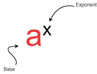
Any exponential function has base and an exponent and keeping this in mind, let me define the exponential function.
Definition Of Exponential Functions
Any function  with base
  is defined as
\begin{aligned} &f(x) = b^x \\ \\
&or \\ \\
&y = b^x
\end{aligned}
where is a positive constant except 1 meaning  and is any real number.
What is not exponential functions?
Consider the following functions.
\begin{aligned}
&f(x) = (-3)^x \\ \\
&f(x) = 1^{x+1}\\ \\
&f(x) = x^x \\\\
&f(x) = x^2
\end{aligned}
You have to remember two rules for exponential functions, (1) base is a positive constant greater than and not equal to (2) exponent is a variable representing real number. The functions above violates one or both rules, hence, they are not exponential functions.
The function  will give negative results for odd values of and positive results for even values of .
For example,  , but
, but  . Therefore, it is not an exponential function.
The next function above,  has proper structure, except that it violates the rule 1,
  .
.
Similarly, the function  and
and  violates rule 1 which says base must be a positive constant, not variable. Also, exponent cannot be a constant which is the violation of rule 2.
Graph Of Exponential Functions
Rational Functions
Rational functions are special functions that you cannot call polynomials, but are obtained by dividing polynomials. In other words, they are the quotients of the polynomial division.
A rational function is of form  where
where  and
and  are polynomials and
 . The domain of rational function can be any real numbers except those that makes
  .
.
Example #1
 is a rational function. The function accept all real number except 1. The value 1 makes the function invalid. Hence, we can write domain of the as
  .
.
Example #2
Find the domain of rational function  .
.
Solution:
The rational function accepts all values, except  , which we can write in interval notation also,
  .
.
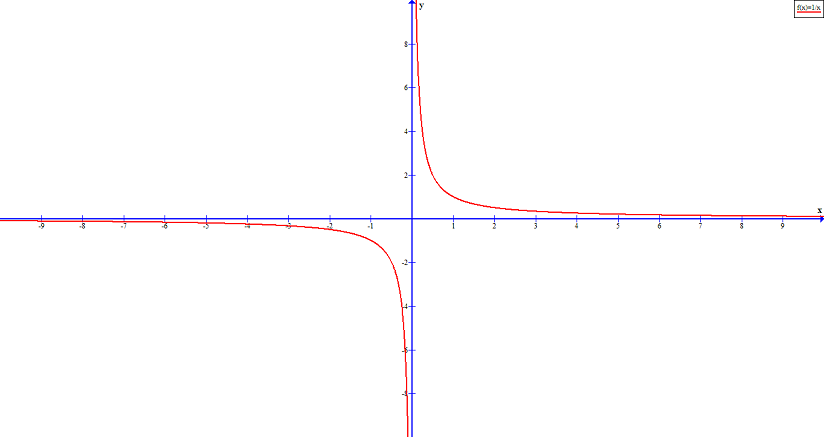
The Reciprocal Function
The simplest of rational function is the reciprocal function  . The function accepts all real values except .
Let us plot the graph of this rational function for following values.
| X | -1 | –0.5 | -0.1 | -0.01 | -0.001 | -0.0001 |
| F(x) | -1 | -2 | -10 | -100 | -1000 | -10000 |
As the value approaches from left, the value of becomes smaller and smaller boundlessly to  . This can be shown with the arrow notation as follows.
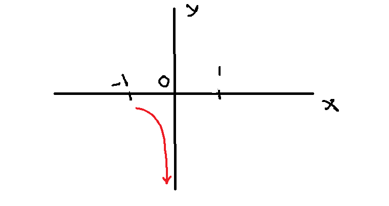
![\[x \to 0^{-} , f(x) \to -\infty\]](https://notesformsc.org/wp-content/ql-cache/quicklatex.com-f9b24cb2bb68526fe693c381970b2d13_l3.png "Rendered by QuickLaTeX.com")
 ,
, 
What happens when comes closer to from right side.
| X | 0.0001 | 0.001 | 0.01 | 0.1 | 0.5 | 1 |
| F(x) | 10000 | 1000 | 100 | 10 | 2 | 1 |
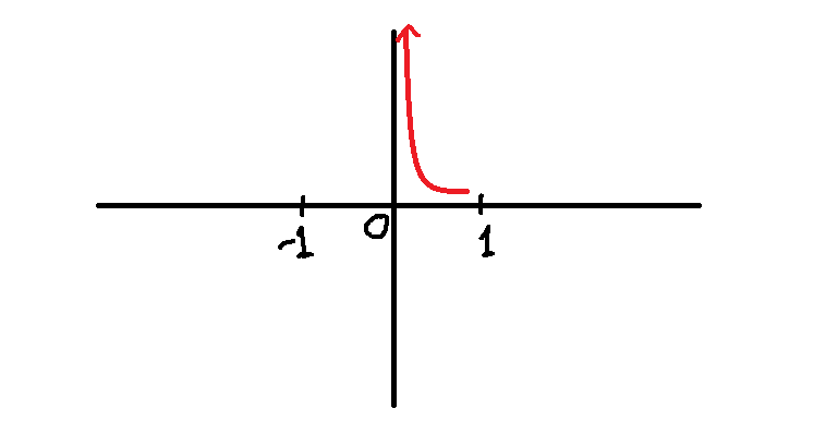
 ,
, .
.
As the value approaches 0 from right , the value of increases boundlessly to positive  . This is shown above with arrow notation.
What happens when the value of moves away from , that is, increases or decreases boundlessly ?
| X | 1 | 10 | 100 |
| F(x) | 1 | 0.1 | 0.01 |
| X | -1 | -10 | -100 |
| F(x) | -1 | -0.1 | -0.01 |
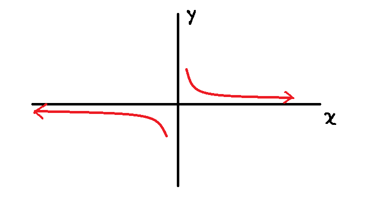
When the value increases or decreases boundlessly, then the approaches , but not touching .
This is shown in arrow notation below.
 ,
,  and
and  , .
, .
Vertical Asymptotes
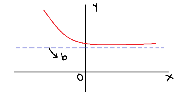
There are several rational functions, out of which  is an interesting one. The graph of this function is reflected across the y-axis.
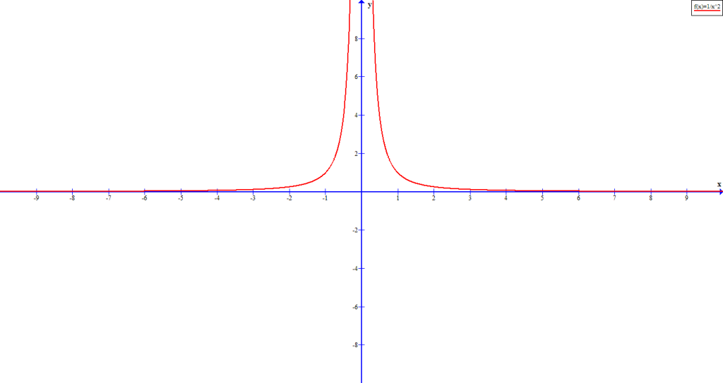
We can describe the end behavior of this graph in the following manner.
| , |  , , |
| , | , |
The line  is called the vertical asymptote of the graph. A rational function can have
- one vertical asymptote
- many vertical asymptotes
- or no vertical asymptotes
The end behavior of rational function around vertical asymptote are:
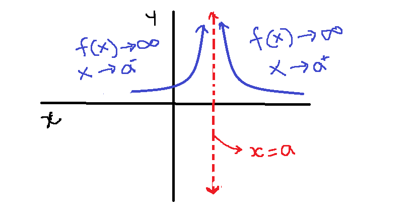
Figure 7 – As x approaches a, f(x) increases boundless
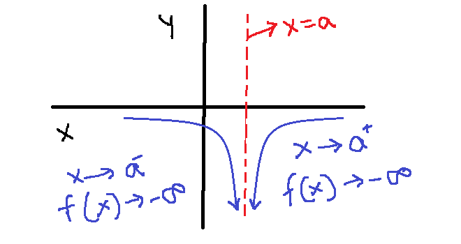
As the value of approaches the  , the increases or decreases without bound.
This increase or decrease in end behavior is useful in study of calculus. We can describe how the value of and the function changes using limits.
The moves closer to from left or right, the end behavior changes is shown in limits below.
 |  |
 |  |
How To Locate The Vertical Asymptotes ?
If the rational function have vertical asymptotes, then it can be found easily. We know that where and are two polynomials. There are two conditions to find the vertical asymptotes:
- The polynomials
 and
and  have no common factors, if they have common factor must be eliminated.
 - The value
 must be zero of the polynomial , that is, denominator. If is zero then
  is the vertical asymptotes.
You can understand this with the help of an example.
Example #3
Find the vertical asymptotes of the rational function: 
Solution:
The given equation does not have any common factors, therefore, meet the first condition. The denominator accepts all real numbers except  which makes it .
Therefore,  is the vertical asymptote in the graph of rational function.
Example #4
Find the vertical asymptote of the rational function:  .
.
Solution:
In the given equation,  has a common factor. We reduce the common factor and the equation becomes
  .
.
The function accepts all real values,  except . Therefore,
  is the vertical asymptotes.
Example #5
Find the vertical asymptotes for the rational function:  .
.
Solution:
The function has no common factor, but there is no value for which the denominator is . Therefore, the function does not have a vertical asymptote.
In some cases, the denominator is shows that it has a zero, but after reducing the common factors, the resultant expression has a totally new vertical asymptote.
Example #6
Find the vertical asymptote for the equation:  .
.
Solution:
At first we see that the equation has a zero  , but when the equation is reduced after reducing the common factors, we get
  and the vertical asymptote is
  .
.
Horizontal Asymptotes
The equation  represents “vertical asymptote“, similarly,
  represents the “horizontal asymptotes“. There may be several vertical asymptotes, but there is only one horizontal asymptote.
The function , as increases or decreases without bound or , the approaches , which is . So, we can say that the horizontal asymptote is that which is defined as  .
.
We can write them in limit form as:
 |  |
Zeros of Polynomial Functions
In the previous article, where we introduce polynomials, a brief introduction to the roots of quadratic equations were discussed with some examples. Now you are going to learn the zeros of polynomial in more detail.
The idea of zero is that to find those x values for which  and it is the x-intercepts in case of quadratic equations which is also a polynomial of degree 2.
Rational Zero Theorem
As we mentioned earlier, the zeros or roots of a polynomial is nothing but those values of for which  .
.
If  is a polynomial with integer coefficients, then
  is the rational zero of the polynomial where
  is the factor of constant term
  and
and  is the factor of leading coefficient
  .
.
This is could be understood with the help of an example.
Example #1
Find the rational zeros of  .
.
Solution:
The constant term is  and its factors are
  .
.
Similarly, the leading coefficient is whose factors are  .
.
Therefore,
Rational Zeros = 

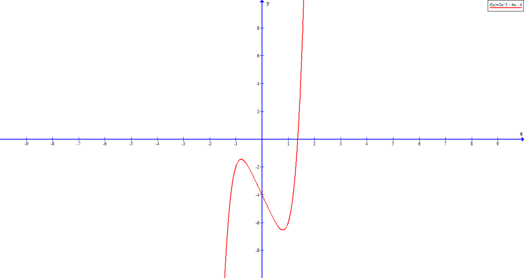
There are total 8 roots for this polynomial equation. The actual roots are .
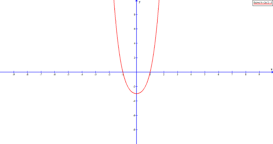 shows root at -1 and 1
How To Use The Rational Zero Theorem?
We can use the rational zeros to find the real zero of the polynomial. Note that the polynomial is divided by  such that .
Example #2
Find the real root of the polynomial  from its rational zeros.
Solution:
The constant term is -3 so the factors of constant terms are  .
.
The leading coefficient term is 1 and the factors of leading coefficient are .
Rational \hspace{2 mm} zeros = \frac{\pm1, \pm3}{\pm1}
= \frac{\pm1}{\pm1}, \frac{\pm3}{\pm1}
=\pm1, \pm3
Now we test each of the root to find the real root of the polynomial. For this we have to use synthetic division. If you are not familiar with the synthetic division, read the previous article.
3 : 1 -1 3 -3
       3 6  27   ( This solution is not suitable because remainder is 24. The remainder should be 0).
    1  2 9  24


1 : 1 -1 3 -3
       1 0  3   ( The real root of the polynomial is 1 ).
    1  0 3  0
After performing a synthetic division we are able to find the real root of the polynomial . You can also plot the graph of the polynomial and then look for root which is x-intercept.
Solving Polynomial Equations
The rational zeros of polynomials are very helpful when the degrees of polynomial equations are higher. Consider the following example.
Example #3
Find the solution to the polynomial equation:  .
.
Solution:
To find solution we must find all the rational roots.
The factors of constant 6 are  and similarly, the factors of leading coefficient is
  .
.
The rational coefficients are  .
.
Synthetic Division
Now we can do synthetic division to find the solution.
1 : 2 -3 -11 6
       2  5 -6  ( 1 is a root of polynomial f(x).
    2  5 -6  0
Now we can write the equation as  and remainder is 0.
Example #4
Find the rational root of the following polynomial:  .
.
Solution:
The factors of the constant terms are  .
.
The leading coefficient has following factors : .
The rational roots are  .
.
Synthetic division
To find the factors we now have to use the synthetic division. First we are going test
1: 1 -2 -6 4
      1  1 -5  ( This has a remainder of -1. We need to have remainder of 0 in the last cell.)
   1  1 -5 -1


2: 1 -2 -6 4
      2  0 -12  ( This has a remainder of -8. We need to have remainder of 0 in the last cell.)
   1  0 -6 -8


-2: 1 -2 -6 4
      -2  8 -4  ( This has a remainder of 0. )
    1 -4  2 0
Therefore, the root of the equation is  and
and  is a factor.
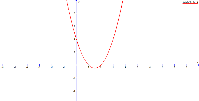
f(x) = (x + 2)(x^2 - 4x + 2)
We can use the quadratic formula to solve  and find rest of the roots.
x = \frac{-b \pm \sqrt{b^2 - 4ac}}{2a} \\ \\
= \frac{4 \pm 2\sqrt{2}}{2} \\ \\
 x = 2 + \sqrt{2}  \hspace{2mm} and \hspace{2mm} x = 2 - \sqrt{2}
Fundamental Theorem Of Algebra
The fundamental theorem of algebra states that a polynomial with a degree  has
has  roots. To understand this consider the following graph.
If is a polynomial with degree where  , then the equation has one complex root.
Example #5
From our earlier example,
We have  we can factor the second degree polynomial using quadratic formula.
 x = \frac{-5 \pm \sqrt{25 - 48}}{4}
= \frac{-5 \pm i\sqrt{23}}{4}
The roots are  and
and  . The complex conjugate is also a root.
Linear Factorization
The linear factorization is states that for a polynomial where  , then the polynomial can be written as product of linear factors, called the linear factorization.
 where
where  are complex numbers.
Example #6
Find the factors of the polynomial:  .
.
Solution:
The factors are 
Using the quadratic formula, 
 x = \frac{-6 \pm \sqrt{36-100}}{2}\\ \\
= \frac{-6 \pm \sqrt{-64}}{2}\\ \\
= \frac{-6 \pm i8}{2} \\
Therefore, the roots are 
We can write the polynomial 
This means that roots are rational , irrational and complex or imaginary numbers. In the next section, we discuss a method to find the real roots for polynomial functions.
Rules of Signs
The rules of signs is also called the Descartes’s rules of signs. In a polynomial with degree , there are at most real roots, the rule of signs provide specific information about the number of real roots in a polynomial equation.
If  is a polynomial with degree with real coefficients, then
number of positive real roots are:
- same as the number of sign changes
 in
in  or
or - less than number of sign change by a positive even integer.
- If there is only one sign change in , then there is only one real root.
 or
ornumber of negative real roots are:
- same as the number of sign changes in
 or
or - less than number of sign change by a positive even integer.
- If there is only one sign change in , then there is exactly one real root.
 in
in  or
or , then there is exactly one real root.
Example #7
Find the number of real roots in the following polynomial:
f(x) = x^3-7x^2+41x-87
Solution:
First we will find the number of sign changes in the given polynomial function.
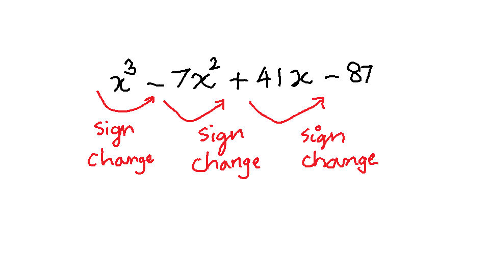
The above equation , there are 3 signs change. Therefore, there are positive real roots of .
Or since, is positive, we have  positive real root.
We can find the zeros of the polynomial to confirm this. The factors of the polynomials are  .
.
How Rules Of Signs Are Helpful In Solving Polynomials?
The rules of signs helps us to eliminate the unwanted roots from all the rational roots. To illustrate this, we use an example.
Example #8
Find the real roots of the following polynomial:  .
.
Solution:
The number of sign change in this polynomial is 3, therefore, real roots are or .
Let us find the rational roots of this equation.
Factors of the constant terms is  .
.
Factors of the leading coefficient is .
Rational \hspace{2mm}roots = \frac{\pm 1, \pm 2 ,\pm 3, \pm 6}{\pm 1} = \pm 1, \pm 2 ,\pm 3, \pm 6The rules of sign inform us that there is no negative real roots in this equation . Therefore, we can eliminate all the negative values. The remaining rational roots are  .
.
Test With Synthetic Division
1: 1 -6 11 -6
      1 -5  6 ( Since, the remainder is zero, 1 is a positive real root of .
   1 -5  6  0


3: 1 -6 11 -6
      3 -9  6 ( Since, the remainder is zero, 3 is a positive real root of .
   1 -3  2  0


2: 1 -6 11 -6
      2 -8  6 ( Since, the remainder is zero, 2 is a positive real root of .
   1 -4  3  0

There are three real roots as per rules of signs.
Summary
In this article, you have learned how to find the rational roots, and under special circumstance such as , there are complex or imaginary roots, so we can find these roots with the linear factorization and rules of signs technique.
Dividing Polynomial Functions
You can divide a polynomial just like numbers and dividing a polynomial will give an expression as quotient and remainder. The polynomial you are going to divide must have more terms than the divisor, else the division will not be fruitful.
In this article, you will learn about polynomial long division and synthetic division techniques.
Polynomial Long Division
To divide a polynomial, you need to follow some steps.
Example #1
Step 1: Keep the terms of the dividend and divisor in standard form, that is, in the descending powers of the variable.
x + 2 )\overline {x^2 + 7x + 10}Step 2: Take first term of the dividend and divide with the divisor, you will get the first term of the quotient. Do it as if you are dividing two numbers.
x\\
x + 2 )\overline {x^2 + 7x + 10}
Step 3: Multiply every term of the divisor with the first term of the quotient.
x\\
x + 2 )\overline{x^2 + 7x + 10}\\
 x^2 + 2x
Step 4: Subtract the result of multiplication in step 3 with dividend.
x\\
x + 2 ) \overline{x^2 + 7x + 10} \\
x^2 + 2x\\
\hspace{1.5 cm}\overline{5x + 10}
Step 5: Bring down the new term from the dividend and repeat the step 1 to 5 until you get a remainder 0 or some other value.
x + 5\\
x + 2 ) \overline{x^2 + 7x + 10} \\
x^2 + 2x\\
\hspace{2 cm}\overline{5x + 10} \\
\hspace{2 cm}5x + 10\\
\hspace{3 cm}\overline{0}\\
The solution to the above polynomial is  which is you obtained after the polynomial long division as quotient. Let perform a polynomial long division on another polynomial.
Example #2:
Divide \hspace{3 mm} x - 1 ) \overline{x^3 + 3x^2 + 3x -4} Solution:
\begin{aligned}
&\hspace{ 1 cm}x^2 + 4x + 7 \\
&x - 1 ) \overline{x^3 + 3x^2 + 3x - 4} \\
&\hspace{ 1 cm}x^3 - x^2  \\
&\hspace{ 1 cm}\overline{4x^2 + 3x } \\
&\hspace{ 1 cm}4x^2 - 4x\\
&\hspace{ 2 cm}\overline{7x - 4} \\
&\hspace{ 2 cm}7x - 7\\
&\hspace{ 2.7 cm}\overline{11}\\
\end{aligned}
This time the solution is a trinomial  . Note that the result of polynomial long division is not always zero, you may get a non-zero remainder too.
How do you write answer when the polynomial long division gives you a remainder. As in above case, you can write answers as
\frac{x^3 + 3x^2 + 3x -4}{x - 1} = x^2 + 4x + 7 + \frac{13}{x - 1}The divisor still tries to divide the remainder so you represent it as a term.
Division Algorithm
We can rewrite the whole dividend , divisor , quotient and remainder as an expression by itself.
x^3 + 3x^2 + 3x -4 = (x - 1)(x^2 + 4x + 7) +11
What we are doing is a check to see whether multiplying and adding the remainder back will give us the original polynomial function
Let say that the dividend is , divisor is  , quotient is and remainder is
  .
.
The degree of divisor is less than or equal to , where  . Also, there exists unique polynomials and .
The degree of remainder is 0 or less than degree of divisor . If remainder  , then we can say that divisor divides polynomial evenly and and are factors of the polynomial.
Synthetic Division
Another way to divide polynomial is much faster and efficient provide that the divisor is in the form  where
where  is a constant.
We can take our previous example to perform the synthetic division.
Example #3
Divide using synthetic division method: 
Solution:
Step 1: Write the constant $c$ from the divisor and all the coefficients from the dividend.
| Divisor c value | 1st term coefficient | 2nd term coefficient | 3rd term coefficient | 4th term coefficient |
| 1 | 1 | 3 | 3 | 4 |
Step 3: Write the 1st term coefficient in third column.
| Divisor c value | 1st term coefficient | 2nd term coefficient | 3rd term coefficient | 4th term coefficient |
| 1 | 3 | 3 | 4 | |
| 1 |
Step 4: Multiply 1st term coefficient with c and write the result in second column and second row and add the entries of second column. Write the result in second column, third row.
| Divisor c value | 1st term coefficient | 2nd term coefficient | 3rd term coefficient | 4th term coefficient |
| 1 | 3 | 3 | 4 | |
| 1 | ||||
| 1 | 4 |
Step 5: Repeat the process from step 1 to 4.
| Divisor c value | 1st term coefficient | 2nd term coefficient | 3rd term coefficient | 4th term coefficient |
| 1 | 3 | 3 | 4 | |
| 1 | 4 | 7 | ||
| 1 | 4 | 7 | 11 |
The numbers in the last row is coefficients of quotient and remainder . Therefore, the result is
q(x) = x^2 + 4x + 7 + \frac{11}{x -1}Remainder Theorem
Let us remember the division algorithm, which is
f(x) = d(x) . q(x) + r
Suppose we are dividing with , then remainder will be a constant  , which means,
f(x) = (x - c) q(x) + r
Given the above equation, suppose  , then
f(c) = (c - c)q(c) + r\\
= 0 \cdot q(c) + r\\
f(x) = r
Therefore, remainder theorem states that you can use from and get the remainder.
Example #4
Find the remainder for  divided by
Solution:
Using reminder theorem,  and
and  .
.
f(1) = 1^3 + 4(1)^2 + 3(1) + 2 = 1 + 4 + 3 + 2 = 10
Therefore, remainder is  .
.
Verify the results:
1 : 1  4  3  2
       1  5  8
    1  5  8  10

Using the synthetic division we find that the remainder is 10.
Factor Theorem
The factor theorem is derived from division algorithm. Suppose the divides the polynomial . We know that by remainder theorem,  which result in .
Let us replace in above equation as  . Now the division algorithm becomes
  .
.
Suppose if the  then, the equation becomes
  which implies that
  is a factor of .
Let us say that is a factor of polynomial .Then,
f(x) = (x - c) q(x) ,  if \hspace{2 mm} x = c\\
f(c) = (c - c) q(c) = 0 \cdot q(c) = 0
If is a factor of , then . This is known as factor theorem.
Summary
In this article, you learned about polynomial long division, synthetic division, division algorithm and two theorem that are derived from the division algorithms – remainder theorem and factor theorem.
Quadratic Functions
Certain functions are symmetric in nature and quadratic function is one of them. If you remember from previous articles, we classified the functions as even and odd which means even functions are symmetric over y-axis and odd functions are symmetric over x-axis in a 2d coordinate plane.
What is a quadratic function ?
A quadratic function is a polynomial function with greatest exponent or degree of 2. Any function of the following form,
f(x) = ax^2 + bx + c
where  are real numbers and
  .
.
We can use the equation above and plot a graph for the quadratic function.
The Parabola
The graph of quadratic function is called the parabola. Since, the quadratic function is even, the graph is symmetric over y-axis. Suppose  is a quadratic function where coefficient
  . Then the quadratic function is . The graph of this function is given below.
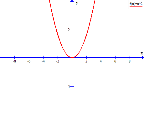
If you notice, the above function can be written as  where
where  . If the coefficient of
  term is greater than 0, that is,
  , then the parabola open upwards.
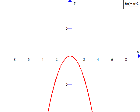
Let us say,  , then quadratic function
  is downward facing.
Whatever may be the type of parabola, certain features are common to all of these parabolas. Let us discuss each on of them.
Features of Parabola
The parabola has certain common features despite various transformations. It does not matter whether graph of quadratic function is wide, narrow, upward facing, or downward facing, these features are always present.
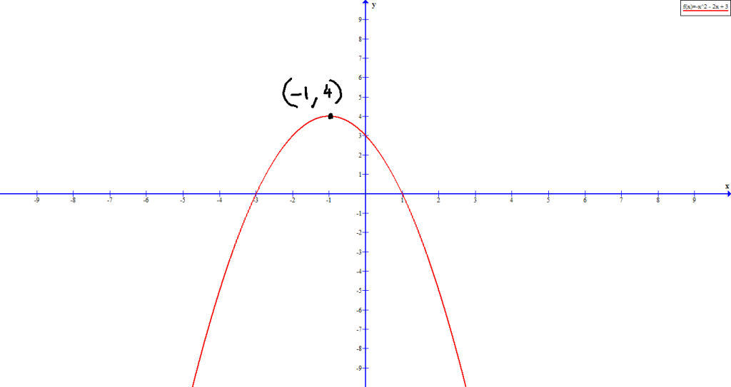
Consider the following quadratic equation,  and its graph.
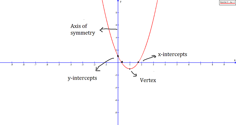
The common features of all parabola are:
- Axis of symmetry
- Vertex
- x-intercepts
- y-intercept
We shall now discuss each of them briefly.
Axis of Symmetry
The axis of symmetry is the y-axis because parabola is graph of a quadratic function which is even. Any even function reflects along the y-axis in a 2D coordinate plane.
Vertex of Parabola
The vertex of a parabola is lowest or the highest point in the graph. When the function is  , which means coefficient
  , then the vertex is at
  on the coordinate plane.
When the parabola is opening upward , the vertex is the lowest point in the graph.
When the parabola open downwards, which is  , the vertex is the highest point on the graph.
Now we know the vertex and parabola features. Note that the graph is transforming, and this gives us a standard form of quadratic equation.
Standard Form of Quadratic Equation And Transformation of Graph
The basic form of quadratic equation is where and  . The vertex of such a graph is at . If we apply transformation on the parabola, whose vertex
  is away from origin
  , we get:
f(x) = a(x - h)^2 + k
where .
Here are some important points to note:
- If
 , then the graph open upwards, else if , then the graph open downwards.
 - The transformed quadratic function from
 has a vertex
  .
. - When the value of
 is positive, the graph shifts unit to the right, and if
  , the graph shifts unit to left.
 - When the value of , then graph shifts upwards in y-axis, otherwise, it shift down k unit along the y-axis.
- The equation of axis of symmetry is
 where is the vertex.
 - The x-intercepts can be calculated by solving the quadratic equation, that is,
 .
. - The y-intercept can be calculated using .
 has a vertex
  is positive, the graph shifts
  , the graph shifts
  , then graph shifts upwards in y-axis, otherwise, it shift down k unit along the y-axis.
 .
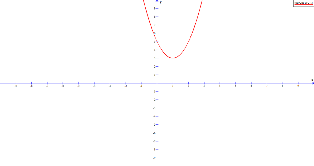
.Let us graph a quadratic equation in standard form.
Example #1
Graph the following quadratic equation:  .
.
Solution:
Before we construct the graph, let us observe a few things about this quadratic equation which is in standard form.
 , which means that the graph open upwards. The vertex is
  .
.
We know that the line of symmetry is  , therefore,
  . Also, the graph shifts upwards 3 units.
The y-intercept is  . There is no x-intercepts in the graph because the graph already shifted 3 units up in the y-axis.
Based on the information above we can construct the graph, which look like the following.
What if we are given equation in the form:  .
.
Graphing Equation Of Form: 
To solve equation of form , we need to change it into standard form. This is achieved through completing the square process.
Example #2
Change the given equation into standard form:  .
.
Solution:
Let the equation be perfect square.
\begin{aligned}
&2x^2 + 4x + 5 = 0\\ \\
&dividing \hspace{2 mm} all \hspace{2 mm}terms\hspace{2 mm} by\hspace{2 mm} 2\\ \\
&=x^2 + 2x + 5/2 = 0 \\ \\
&=(x^2 + 2x + 1) -1 + 5/2 = 0\\ \\
&Completing\hspace{2 mm} square \hspace{2 mm}and \hspace{2 mm}multiply \hspace{2 mm} by\hspace{2 mm} 2\\ \\
&=2(x + 1)^2 - 2 + 5 = 0 \\ \\
&=2(x + 1)^2 + 3 = 0
\end{aligned}
Now, in the standard form, it is easy to graph the equation. The vertex of the above equation is  . However, there is an easier way to get coordinates for vertex,
If , then its vertex is  , where
\begin{aligned}
&h = \frac{-b}{2a}\\\\
& f\left(\frac{-b}{2a}\right)
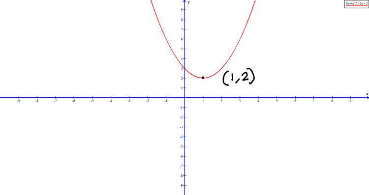
\end{aligned}Example #3
Find the vertex of equation: .
Solution:
Vertex is
\begin{aligned}
&h = \frac{-4}{4} = -1 \\\\
&k = f(-1) = 2(-1)^2 + 4 (-1) + 5 = 2 - 4 + 5 = 3

\end{aligned}
Therefore, the vertex is .
Maximum and Minimum Points
The quadratic equation problems are find three values starting point, maximum or minimum point on the graph, and ending of the graph. The x-coordinate value of vertex gives the location of maximum or minimum point, and y-coordinate value gives the value of maximum or minimum point in the graph of quadratic equation.
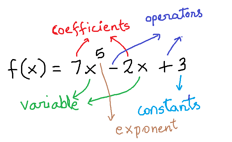
Polynomial Functions
In this article, you will learn about a special function called polynomial function. You can think of polynomials as an expression made of variables, exponents, and constants. Here the number of terms are important, hence, the name “Poly” which means “many” and “nomial” means “terms”.
Standard Form
The standard form of polynomial function is in following form.
\begin{aligned}
&f(x) = a_nx^n + a_{n-1}x^{n-1} + ... + a_2x^2 + a_1x + a_0\\ \\
&where\\\\
&;a \neq 0, n \geq 0 \hspace{2 mm} and \hspace{2 mm} \{ a_n, a_{n-1}, ... , a_2, a_1, a_0 \} \in R
\end{aligned}
The value is non-negative integer and it is called the degree of polynomial function. The value is leading coefficient for variable with highest power, that is,  . Finally, all coefficients are real numbers.
What Is Not Polynomial Function ?
As we mentioned earlier, the coefficients can be any real number, however, the exponents value must be a non-negative integer.
Example #1

The function  is a polynomial of degree
  because the variable has non-negative integer exponent and the coefficients are real numbers. The negative numbers and radicals are also real numbers.
Example #2

The function  is not a polynomial function because it has a fraction exponent, it must be a non-negative integer exponent.
Example #3

The exponent in the leading term has a negative value, all exponent in polynomial must be greater than or equal to 0, meaning a non-negative integer.
Polynomial Types Based on Number Of Terms
The terms of polynomial are separated by arithmetic operators such as plus (+) and minus (-). Based on number of terms a polynomial can be classified into:
- Monomial
- Binomial
- Trinomial
Monomial
A monomial is a single term polynomial. A single term can be a constant or a term with variable.
Example #4
 where
where  .
.
Note that the variable is  therefore,
  , and it is also known as constant polynomial.
Example #5
 where .
Binomial
If the polynomial has only two terms, then it is known as a binomial.
Example #6
 where .
The above is example of binomial polynomial, but the degree is one. Such a polynomial is called linear function.
Trinomial
The trinomials have three terms.
Example #7
 where
where
These type of polynomial are trinomials and a trinomial with degree two is called a quadratic equation. You can read previous article to know more about quadratic functions.
Graph Of Polynomial Functions
The graph of polynomial function has two characteristic:
- The graph is continuous, meaning it has no breaks.
- The graph is smooth, meaning the graph is a single function with out sharp edge.
A continuous function can be a piecewise function which is not graph of polynomial.

You can recognize the graph of a polynomial just by looking at the smoothness and continuity. Any sharp corner in graph is not a polynomial function.
End Behavior of Polynomial Functions
If you notice that the graph of polynomial has two ends – rightmost end and leftmost end. The end behavior depends on what kind of polynomial we are dealing with. The graph may go up or down during intervals, but the ends behavior depends of a polynomial  depends on
- coefficient
 of the leading term
  in the polynomial.
 - value of exponent
 in the leading term .
 in the polynomial.
You can see from the figure 2, that when the value of variable increases, only leading term dominates , all smaller terms are insignificant. Therefore, we perform a leading coefficient test to determine the end behavior of the polynomial function.
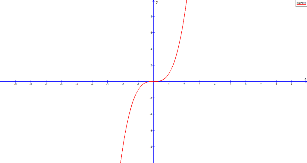
When is odd:
 (positive) (positive) | left end decreases | right end increases |
 (negative) (negative) | left end increases | right end decreases |
 value and positive value.
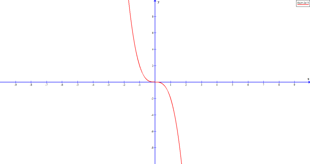 value and negative value.
When is even:
| (positive) | left end increases | right end increases |
| (negative) | left end decreases | right end decreases |
The even polynomial has both ends pointing to same direction.
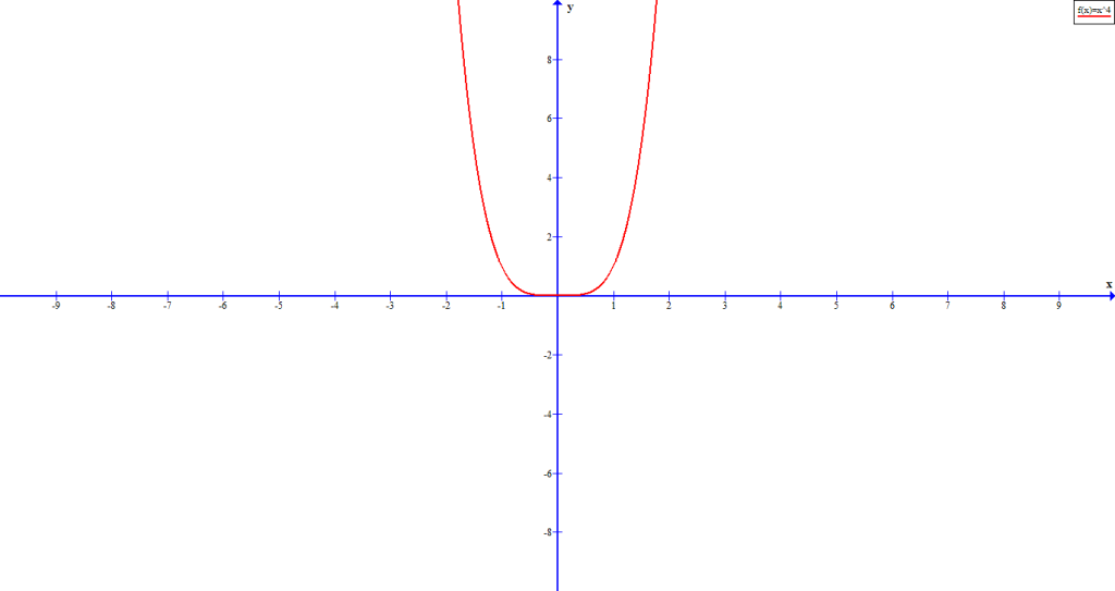 and positive value
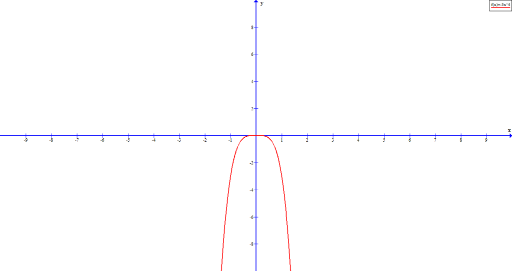 and negative value
Figure 6 is graph of  and figure 7 is graph of
  .
.
Example #8
Determine the end behavior of the following function:  .
.
Solution:
From the graph above it is easy to understand that this is an odd polynomial function with degree  . The leading coefficient is
  which is greater than 0, that is, .
Therefore, the graph of has leftmost end decreasing and rightmost end increasing as variable increases without bound.

Zeros Of Polynomial Function
If is a polynomial function, then value of for which is called zero of polynomials. There can be more than one zeros of a polynomial function.
The zeros of a polynomial function are called roots or solutions to the function . They appear as x-intercept in the graph of a polynomial function.
Example #8
Find the zeros of the polynomial:  .
.
Solution:
This problem cannot be solved with grouping technique. So checking whether  is a solution.

Therefore, is a solution.
Using we can perform a polynomial division to find the roots.
\begin{aligned}
&\frac{x^3 +5x^2 + 8x + 4}{x + 1} = x^2 + 4x + 4 = (x + 2)^2
\end{aligned}
Therefore, the roots are and  .
.
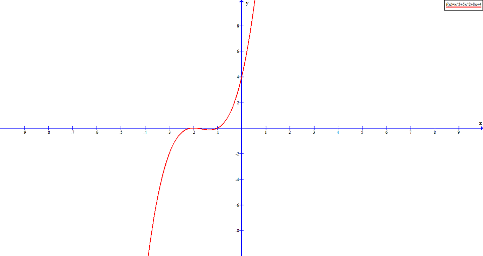
 is at and
Multiplicities of the Root
In the above example, the root  is repeated two times and not crossing the x-axis The graph shows that root which crosses the x-axis. This is called multiplicity of the root.
- If the multiplicity of the root is even, that means if the root repeat itself even times, it does not cross the x-axis.
- If the multiplicity of the root is odd, then the root cross the x-axis.
The reason why graph does not cross the x-axis when the multiplicity is even is because when the multiciplity is even, the sign of the does not change at all.
Example #9
Consider the following graph of  which has two roots
  and . The factors of the function are
  .
.
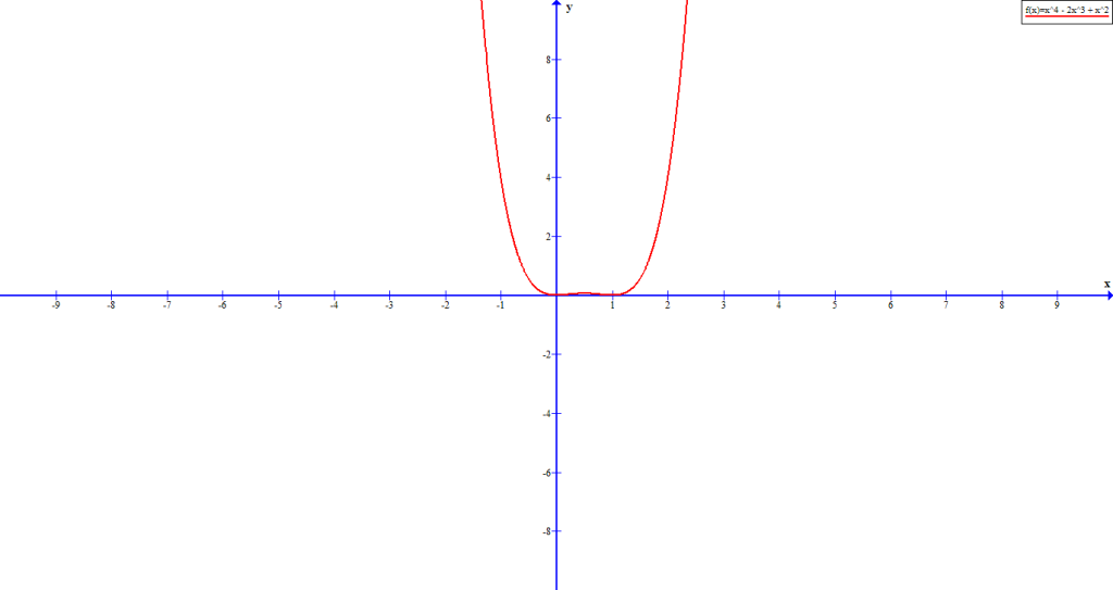
The graph clearly shows that the function does not cross the the x-axis at or .
Example #10
In this example, we have a polynomial function :  whose factor is
  . The x-intercept is .
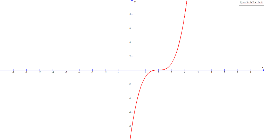
The graph crosses the x-axis at because the multiplicity of the root is odd.
A polynomial function is a function of the form
where is a non-negative integer and .
The degree is the highest power of the variable with a non-zero coefficient.
Polynomial functions are classified as constant, linear, quadratic, cubic, etc., based on their degree.
No. A polynomial function can have only non-negative integer powers of the variable.
Q5. What are zeros of a polynomial function?
They are represented by smooth, continuous curves with no breaks or sharp corners.
They are widely used in mathematics, science, and engineering to model real-world relationships.
Understanding Limits and Continuity
Limits and continuity of function is where calculus topics starts, however, to know calculus you must complete all lessons of pre- calculus with examples.
Limit of a function is a certain value that a function approaches, whereas a function is said to be continuous when the function has no breaks or drawn without taking the pen away from the paper.
How to understand a limit of a function?
Limit of a function is a certain value on x- axis that a function of x approaches from both the sides. When a function of x approaches to n (where n is an integer), then all the values of x are very close to n from both the side of the number line. For example, when function of x approaches to 2, then the the values near to the limit of a function from the left if 1.9, 1.99, 1.999 etc. and from the right is 2.1, 2.01, 2.001 etc.
Limit with an example
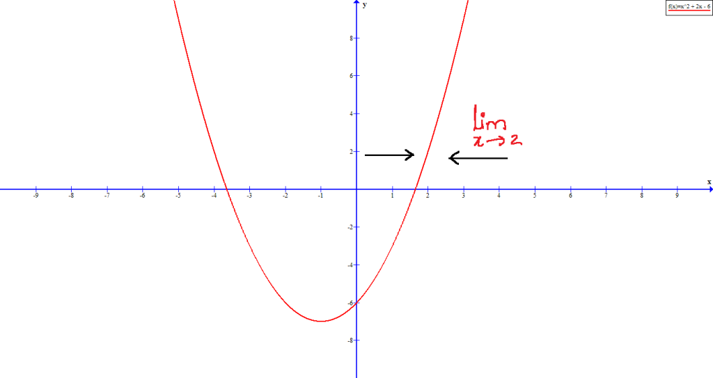
Let us say $latex f(x) = x^{2} + 2x – 6$ is a function whose limit is 2, then, the limit of a function can be written as $latex \displaystyle \lim_{x \to 2}&s=1$. This can be showed in the form of a graph.
While finding the limit of a function, what should we observe?
Finding the limit of a function is all about observing the particular value a function approaches from left and right. From figure 1, it can be observed that both the right hand limit and left hand limit of a function approaches to the same number. In the above graph, the limit approaches from both right and left to 2.
$latex \displaystyle \lim_{x \to c^-}&s=1$ means that x approaches c from left and reach all numbers smaller than c.
Similarly,
$latex \displaystyle \lim_{x \to c^-}&s=1$ means that x approaches c from right and reach all numbers greater than c.
Note: the value of x is never equal to c.
Continuity of a function
The limits applies to a continuous function. If the function is continuous, then a limit exists, otherwise not.
What is continuity of a given function?
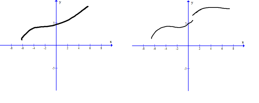
A function is said to be continuous, when graph for the given function shows no breaks or discontinuity at a point or at least in a given interval.
How to find whether a function is continuous?
Continuity of a function can be examined in two ways.
- Continuity of a function at a given point
- Continuity over a given interval
For finding the continuity of is given function is, the given function should have no breaks at the neighbourhood to a given point.
How to determine the continuity of a function at a given point?
For checking the continuity of a function at a given point, then it must satisfy the following conditions viz.,
- The point at which continuity of a function is examined should be within the domain of the function.
- Both the left handed and right handed limit of the function approaching to the point should be equal.
Summary
- Limit of a function is approached from both the sides.
- If the difference between the nearest value and the limit n is $latex h, h_{1}, h_{2}&s=1$ etc., then the values approaching from the left is $latex n – h, n – h_{1}, n – h_{2}&s=1$.
- In the same case, the values approaching from the right is $latex n + h, n + h_{1}, n + h_{2}&s=1$ .
- Continuity is defined as a function without any breaks or jumps.
Complex Numbers
Complex numbers are extended number system. The motivation behind complex number is that there is no solution to negative roots. Consider the equation  , there is no that can satisfy this equation.
Powers Of Imaginary Number i
Therefore, the imaginary number  is introduced as the solution to
  .
.
\begin{aligned}
The \hspace{1mm}imaginary \hspace{1mm} number \hspace{1mm} i = \sqrt{-1}, where \hspace{1mm} i^2 = -1
\end{aligned}
Now, it is possible to find square root of any negative number.
Example #1
Find the square root of  .
.
Solution:
The square root of a negative number is possible using complex number .
\begin{aligned}
&\sqrt{-64} = \sqrt{(-1) \cdot 64}\\ \\
&= \sqrt{-1} \cdot \sqrt{64}\\ \\
&= i \cdot 8\\ \\
&\therefore \sqrt{-64} = 8i
\end{aligned}
There are few things to note here, firstly, the product property of square roots does not apply for negative numbers, meaning  only works when
  . Since, we are able to use an imaginary number, it is fine to use the product property of square roots.
Secondly, you must write imaginary number to the left of any radical. For example,  is the right way, and
  will create confusion. You can write imaginary number to the right of a real number. For example,
  .
.
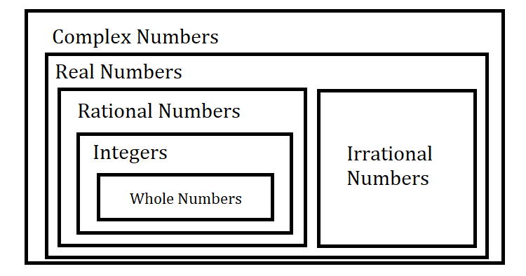
What is a complex number ?
Complex number is extended number system. In a complex number , there are two parts – real part and imaginary part. Therefore, real numbers are subset of complex numbers as shown in the following figure.
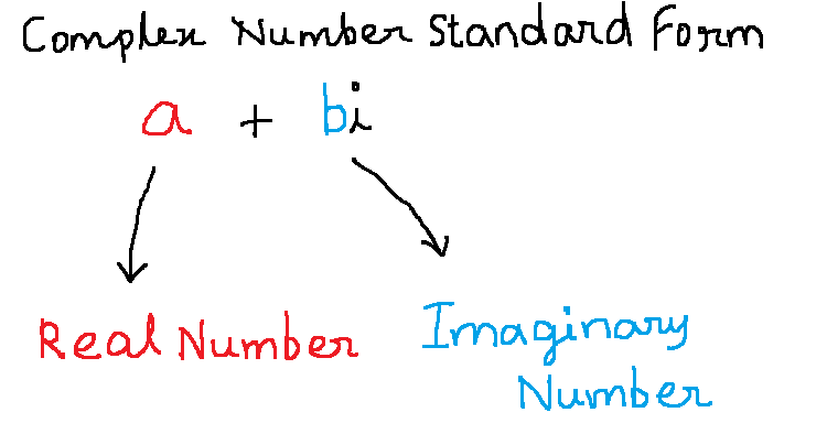
A standard form of complex number is  where is real number and
  is imaginary part of the complex number.
Real Part Of Complex Numbers
Any real number is a complex number of the form where  . We can rewrite this complex number as
  .
.
Imaginary Part Of Complex Numbers
The imaginary part is called pure imaginary number when the real number  , therefore, we can write the pure imaginary numbers as
  .
.
Equality Of Complex Numbers
Complex numbers are equal if their real part and imaginary part are equal. Suppose and  are two complex numbers, then
\begin{aligned}
&a + bi = c + di\\ \\
&If \hspace{2mm} and\hspace{2mm} only \hspace{2mm} if \\ \\
&a = c \hspace{2mm}  and\hspace{2mm}  b = d\\
\end{aligned}
Adding And Subtracting Two Complex Numbers
To add complex number is simple because you need to add the real parts and imaginary parts of two or more complex numbers separately. If and are two complex numbers, then their addition is
\begin{aligned}
&(a + bi) + (c + di) = (a + c) + (b + d)(i)\\
\end{aligned}
Similarly, subtracting two or more complex number requires us to subtract the real parts and the imaginary parts separately. If and are two complex numbers in standard form, their subtraction is
\begin{aligned}
&(a + bi) - (c + di) = a + bi - c - di\\ \\
&=(a -c) + (b - d)(i)
\end{aligned}
We will look at some examples to understand this better.
Example #2
Add the following complex numbers and write results in standard form:  .
.
Solution:
\begin{aligned}
&(3 + 5i) + (7 + 2i)\\ \\
&=(3 + 7) + (5 + 2)(i)\\ \\
&=10 + 7i
\end{aligned}
Example #3
Subtract the following complex numbers and write results in standard form:  .
.
Solution:
\begin{aligned}
&(5 + i) - (6 + 3i)\\ \\
&(5 - 6) + (1 - 3)(i)\\ \\
&-1 + (-2)(i)\\ \\
&-1 -2(i)
\end{aligned}
Multiplying Complex Numbers
Multiplying two complex number is similar to multiplying any algebraic expression except that you have to remember the powers of “iota”. Suppose and are two complex numbers then their multiplication is
\begin{aligned}
&(a + bi)(c + di) = ac + adi + bci + bd(i \cdot i)\\ \\
&= ac + (ad + bc)i - bd\\ \\
&=ac - bd + (ad + bc)i
\end{aligned}
The real terms and the imaginary terms are multiplied separately. This results in square of “iota” in one of the terms which is .
Therefore, multiplication of two complex number results in another complex number.
There are two types of multiplication methods for complex numbers. First is multiplication by distribution method and second is multiplication as you multiply binomials( using FOIL method).
Example #4 : Distribution method
Multiply the following:  .
.
Solution:
\begin{aligned}
&3i ( 2 + 7i ) = 3i \cdot 2 + 3i \cdot 7i\\ \\
&= 6i + 21i^2\\ \\
&= 6i + 21(-1) \hspace{1 cm} i^2 = -1\\ \\
&= 6i - 21\\ \\
&= -21 + 6i
\end{aligned}
In the above example, the term  is distributed to terms inside of the parentheses. Also, the result is a complex number
  which we write in standard form.
Example #5 : FOIL method
Multiply the given complex numbers using FOIL( first, outside, inside, last) method:  .
.
Solution:
\begin{aligned}
&(2 + 5i)(9 + 3i) = 2 \cdot 9 + 2 \cdot 3i  + 5i \cdot 9 + 5i \cdot 3i \\ \\
&= 18 + 6i + 45i + 15i^2 \\ \\
&= 18 + (6 + 45)i + 15 (-1) \hspace{1 cm} i^2 = -1 \\ \\
&= 18 + 51i - 15\\ \\
&= 18 - 15 + 51i\\ \\
&= 3 + 51i
\end{aligned}
Therefore, multiplication by both method- distribution and FOIL result in a complex number when we multiply any two or more complex numbers. Another interesting feature of multiplication of complex number is complex conjugate, about which you will learn in the next section.
Complex Conjugate
The complex conjugate of complex number is  , similarly, complex conjugate of is .
Remember the difference of square in algebra, where  , similarly, multiplying complex conjugates will result in real numbers.
\begin{aligned}
&(a + bi)(a - bi) = a^2 -abi + abi - b^2(i^2)\\ \\
&=a^2 - b^2(-1)\\ \\
&=a^2 + b^2\\ \\
&Similarly,\\ \\
&(a -bi)(a + bi) = a^2 + b^2
\end{aligned}
Clearly, multiplication of complex conjugates results in a real number  .
.
Example #6
Find the complex conjugate and product of the complex conjugates of  .
.
Solution:
\begin{aligned}
&The \hspace{5px}complex \hspace{5px}conjugate \hspace{5px}of \hspace{5px}3 - 2i \hspace{5px}is \hspace{5px}3 + 2i\\ \\
&The\hspace{5px} product \hspace{5px}of \hspace{5px}complex \hspace{5px}conjugates:\\ \\
&(3 - 2i)(3 + 2i) = 9 - 4 (-1) \hspace{1 cm}\because i^2 = -1\\ \\
&=9 + 4 \\ \\
&=13\\ \\
\end{aligned}
The complex conjugates are very important because it help use to solve division involving complex numbers.
Division of Complex Numbers
Imagine that you are dividing two complex numbers, then the goal of the division should be to obtain a real number in the denominator because we are trying to simplify the expression.
If two complex number, and are given then you must use complex conjugate of denominator to simply the expression.
\begin{aligned}
&\frac{a + bi}{c + di} = \frac{a + bi}{c + di} \cdot \frac{c - di}{c - di}\\ \\
&=\frac{ac -adi + bci  + bd}{c^2 + d^2} \\ \\
&=\frac{ac - (ad - bc)i  + bd}{c^2 + d^2}
\end{aligned}
You can see from the above example, that by multiplying with complex conjugate of denominator we get a real number in the denominator.
Application Of Complex Number in Solving Quadratic Equations
The quadratic equation is an equation of following form:  where are real constants. The solution of quadratic equation is given by the formula:
\begin{aligned}
&x = \frac{-b \pm \sqrt{b^2 - 4ac}}{2a}
\end{aligned}
The expression  is called the determinant of a quadratic equation.
- If the determinant is greater than 0, , we have real and distinct roots as solution to quadratic equation.
- If the determinant is equal to 0,
 , we have real and equal roots for solution.
 - If the determinant is less than 0, , we have imaginary roots.
 , we have real and distinct roots as solution to quadratic equation.
 , we have real and equal roots for solution.
 , we have imaginary roots.
When the roots are imaginary , we can solve it using the complex numbers.
Example #7
Solve the following quadratic equation: 
Solution:
We can use the quadratic formula to solve this quadratic equation.
\begin{aligned}
&x = \frac{-2 \pm \sqrt{4 - 20} }{2}\\ \\
&= \frac{-2 \pm \sqrt{-16} }{2}\\ \\
&Therefore, \hspace{2mm}roots \hspace{2mm}are:\\ \\
&\frac{-2 + 4i }{2} \hspace{2mm} ,\frac{-2 - 4i }{2}
\end{aligned}
This is just one of the benefit of complex numbers, there are plenty of situations where complex number are helpful in solving, what is otherwise, not possible with only real numbers.
Equations of Circle
In this article, you will learn about distance formula , midpoint , and equations of circle. The circle is a geometric shape that has a special significance in mathematics. To study the circle, in algebraic form, we need to define it in terms of coordinates in a 2d coordinate system also known as Cartesian coordinate system.
Coordinate System
You are familiar with the 2d coordinate system already from previous articles. The 2d coordinate system define an point in terms of an ordered pair  from origin . The represents horizontal distance from 0 and
  represents vertical distance from .
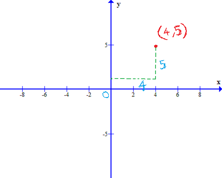
In the figure 1 above, the point  is units in horizontal direction from and units in vertical direction from . Therefore, we must study the circle as a set of points in this 2d coordinate system.
Distance Formula
The distance formula is derived from Pythagorean theorem to find the distance between two points in the coordinate system. Suppose that  and
and  are two points in the
  plane.
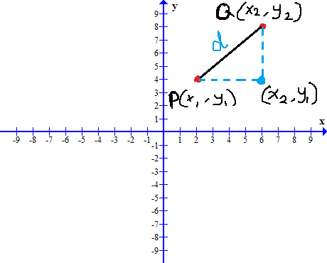
The distance between point to point involve change of value from  to
to  value and change in value from
  to
to  . This forms a right triangle in the plane.
The distance  is hypotenuse of this right triangle and
  and
and  are the lengths of sides of this right triangle. Therefore, by Pythagorean theorem,
\begin{aligned}
&d^2 = (x_1 - x_2)^2 + (y_1 - y_2)^2\\ \\
&Take \hspace{2mm} square \hspace{2mm} root \hspace{2mm} of \hspace{2mm} both\hspace{2mm}  sides. \\ \\
&\sqrt{d^2}= \sqrt{(x_1 - x_2)^2 + (y_1 - y_2)^2} \\ \\
&d =\sqrt{(x_1 - x_2)^2 + (y_1 - y_2)^2}
\end{aligned}
The distance formula is  .
.
Note that the length or  does not matter as long as we take
  or
or  . Similarly, we must take positive value, which is
  or
or  .
.
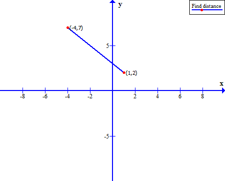
Example #1
Find the distance between point  and
and  .
.
Solution:
Solution:
\begin{aligned}
&Let \hspace{1mm} x_1 = -4 \hspace{1mm} and \hspace{1mm} y_1 = 7,\hspace{1mm}\\
&also \hspace{1mm}x_2 = 1 \hspace{1mm}and\hspace{1mm} y_2 = 2. \hspace{1mm}Then, \\
&(-4) - 1| = |-5| = 5 \hspace{1mm} and \hspace{1mm} |7-2| = |5| = 5
\end{aligned}
The distance between and is:
\begin{aligned}
&d = \sqrt{5^2 + 5^2}\\ \\
&d = \sqrt{50}\\ \\
&d = \sqrt{25 \cdot 2}\\ \\
&d = \sqrt{25} \cdot \sqrt{2}  \hspace{1cm} By Rule \sqrt{ab} = \sqrt{a} \cdot \sqrt{b}, {a,b} > 0\\ \\
&d = 5\sqrt{2}
\end{aligned}
Mid-Point Formula
Given any two point on the plane, you can find the mid-point  . If and
  are two points on the plane.
Then the mid-point formula is given as
\begin{aligned}
M(x, y) = \left( \frac{x_1 + x_2}{2},\frac{y_1 + y_2}{2}\right )
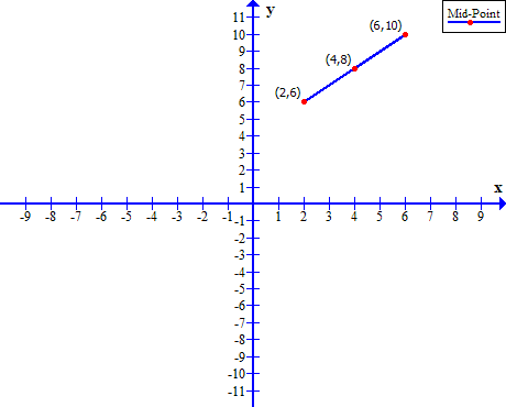
\end{aligned}Example #2
Find the mid-point of points  and
and  .
.
Solution:
We can easily find the mid-point using the mid-point formula, which is  . Given points – and
  .
.
\begin{aligned}
&Let \hspace{2mm} x_1 = 2, \hspace{2mm}  and \hspace{2mm}  x_2 = 6\\ \\
&Similarly, \\ \\
&y_1 = 6,\hspace{2mm}  and \hspace{2mm} y_2 = 10\\ \\
&Using \hspace{2mm} mid-point \hspace{2mm} formula, \hspace{2mm}  get \\ \\
&M(x, y) = \frac{2 + 6}{2}, \frac{6 + 10}{2}\\ \\
&=\frac{8}{2},\frac{16}{2}\\ \\
&=(4,8)
\end{aligned}
Therefore, the mid-point  .
.
Standard Equation of Circle
A circle on the plane is set of all points that equidistant from a fixed point called the center of the circle. The equal distance between center and any point on the circle is called a radius.
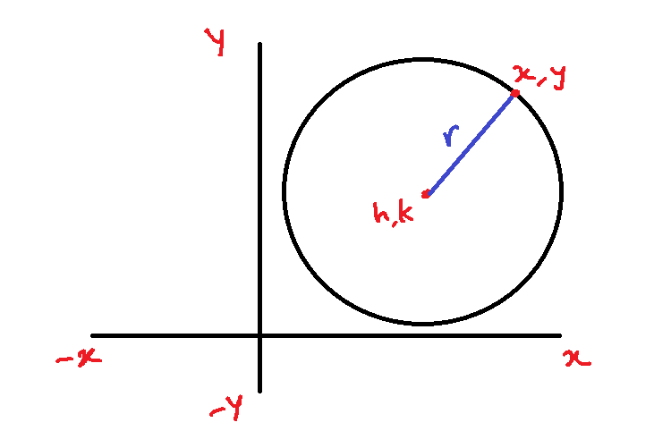
Consider the circle in figure 5, with radius and center at . The point lies on the circle. Therefore, by distance formula, we know that,
\begin{aligned}
&r = \sqrt{(x-h)^2 + (y - k)^2}\\
\end{aligned}
This is the standard equation of a circle with center at .
Circle With Center At The Origin
In the co-ordinate system, the origin is point . A circle whose center is at  has the following equation.
\begin{aligned}
&r = \sqrt{(x - 0)^2 + (y - 0)^2}\\ \\
&r = \sqrt{x^2 + y^2}\\ \\
&or\\ \\
&r^2 = x^2 + y^2
\end{aligned}
Example #3
Find the radius of a circle whose center is at and the point  lies on the circle.
Solution:
Given center  and a point
  , we can use the standard equation of the circle to find the length of radius .
\begin{aligned}
&r = \sqrt{(x-h)^2 + (y - k)^2}\\ \\
&r = \sqrt{(7-1)^2 + (10-2)^2} \\ \\
&r = \sqrt{6^2 + 8^2}\\ \\
&r = \sqrt{36 + 64}\\ \\
&r = \sqrt{100} \\ \\
&r = 10 \hspace{2mm}
\end{aligned}
Therefore, the length of radius is for circle whose center is at and is a point on the circle.
Example #4
Find the center of the circle whose radius and the point  . Also,
  .
.
Solution:
We are given the value of radius  and the point
  on the circle. To find the center point of the circle, we must use the distance formula which is
  and the value of
\begin{aligned}
&r = \sqrt{(x-h)^2 + (y-k)^2}\\ \\
&5= \sqrt{(6 - h)^2 + (8-k)^2}\\ \\
&But, \hspace{2mm} k = h + 1 \\ \\
&5= \sqrt{(6 - h)^2 + (8-(h+1))^2}\\ \\
&5 = \sqrt{(6 - h)^2+ (7 - h)^2)}\\ \\
&5 = \sqrt{36 - 12h + h^2 + 49 - 14h + h^2}\\ \\
&5 = \sqrt{85 - 26h + 2h^2 }\\ \\
&Square \hspace{2mm} both\hspace{2mm}  sides \\ \\
&25 = 85 - 26h + 2h^2 \\ \\
&2h^2 - 26h + 85 - 25 = 0\\ \\
&2h^2 - 26h + 60 = 0\\ \\
&h^2 - 13h + 30 = 0 \\ \\
&(h - 3) (h - 10) = 0\\ \\
&By \hspace{2mm} zero\hspace{2mm}  product \hspace{2mm} property\\ \\
&\therefore x = 3 \hspace{2mm} or \hspace{2mm}  x = 10
\end{aligned}
We try to use the value of in the equation. It seems that  seems more appropriate. Let us verify.
\begin{aligned}
&5 = \sqrt{(6-3)^2+(8-4)^2}\\ \\
&5 = \sqrt{3^2 +4^2 }  \hspace{1cm}  \because k = h + 1 = 3 + 1 = 4\\ \\
&5 = \sqrt{9 + 16}\\ \\
&5 = \sqrt{25 }\\ \\
&\therefore 5 = 5
\end{aligned}
General Equation Of Circle
Suppose a circle has center at  with a point on the circle . Therefore, we can find the standard equation of the circle using,
\begin{aligned}
&r^2 = (x - h)^2 + (y - k)^2\\ \\
&r^2 = (x - 3)^2 + (y - 7)^2\\ \\
&r^2 = x^2 - 6x + 9 + y^2 - 14y + 49\\ \\
&r^2 = x^2 + y^2 - 6x - 14y + 58
\end{aligned}
Therefore, the general equation of circle is  where
where  are real constants.
Example #5
Given the general equation of circle  find the coordinates for center of the circle.
Solution:
Given general equation of circle. We will solve it step-by-step. First group the similar variables together and move constant to the right side of the equation.
\begin{aligned}x^2 - 6x + y^2 -14y = - 58\end{aligned}Now solve for and by completing the square. Note that you have to add same value on both side of the equation.
[\begin{aligned}(x^2 - 6x + 9 ) + (y^2 - 14y + 49) = - 58 + 9 + 49\end{aligned}The equation is in standard form and we can find the value of easily.
[\begin{aligned}(x - 3)^2 + (y - 7)^2 = 0^2\end{aligned}The center of the circle is at  .
.
Inverse Functions
In the previous article, you learned about composite function, in this article, you will learn about inverse functions. The term “inverse” means to “undo” something and which is what the “inverse” of a function do. If a function find the value for an value, the inverse of the function does the opposite, meaning it finds the value for a given value.
Function and its inverse
Remember from previous articles, that the function is set of ordered pair  , that is, for every input there is a one and only .
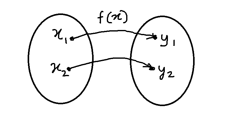
Suppose  is function that takes input and gives us the value . We are just undoing the function . Therefore, if is inverse function of , then it is denoted as
  .
.
The inverse of the function is the set of ordered pairs  .
.
One-To-One Relationship
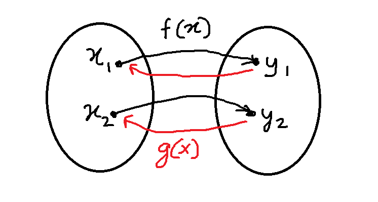
If you look at the figure 2, you will find that there is a one-to-one relationship between function and its inverse  .
.
If there are two functions and its inverse function , then

Where is all values in the domain of inverse function . Similarly,

Where is all values in the domain of function .
If a function does not maintain the one-to-one relationship, there is no inverse. Consider the quadratic function . The function has same outputs for  and
and  .
.
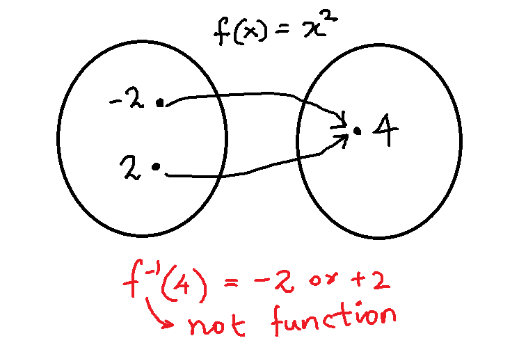
If we take an inverse of the function which is  implies that there are two values for
  . Therefore, inverse is not a function because a function can only have one output for given input .
Horizontal Line Test
The easiest way to understand whether a function has inverse or not is to perform a horizontal line test on the graph of the function. To understand this concept , we will use our previous example of quadratic function . The graph of function is given below.
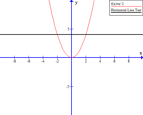
We perform a horizontal line test , that is, draw a horizontal line and if the line intersect the graph of function it has no inverse function. The figure 4 above, shows that the horizontal line intersect the graph of parabola, at  and
and  . Therefore, has no inverse.
Graph of Inverse Function
The graph of inverse function, if exists, can be obtained easily by changing the set of ordered pair to the set of ordered pair .
For example, consider the graph of exponential function  which is an exponential function. The function passes the horizontal line test, therefore, an inverse function exists.
| x | f(x) =2^x |
| -4 | 0.0625 |
| -3 | 0.125 |
| -2 | 0.25 |
| -1 | 0.5 |
| 0 | 1 |
| 1 | 2 |
| 2 | 4 |
| 3 | 8 |
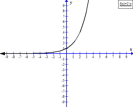
The inverse function is set of all ordered pairs . The inverse function of exponential function is  .
.
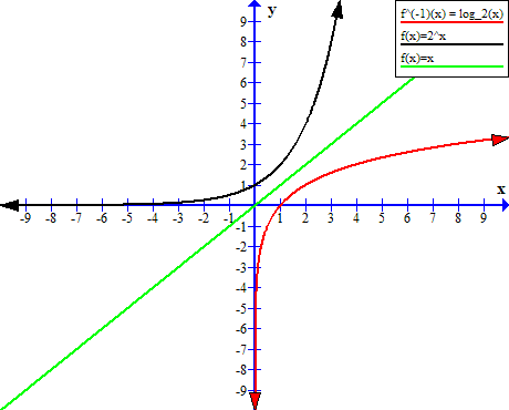
| x | f^{-1}(x) |
| 0.0625 | -4 |
| 0.125 | -3 |
| 0.25 | -2 |
| 0.5 | -1 |
| 1 | 0 |
| 2 | 1 |
| 4 | 2 |
| 8 | 3 |
Note that the inverse function is accepting all positive values, and all inverse function (shown in red) will reflect over the line ( in green)  . The ordered pairs in exponential function is replaced with ordered pair
  .
.
How To Find The Inverse Function ?
To find the inverse of the function you must follow the following steps. If is a function with an expression, then
- Write
 instead of .
 - Interchange the
 and in the equation.
 - Solve the equation for and if the equation does not define in terms of , then there is no inverse. Otherwise, you will have an equation that defines in terms of .
- Replace with
 .
.
Now, it is necessary to verify the inverse function, that can be done by verifying  and
and  . The composition of
  and
and  is an algebraic proof of inverse function.
Example #1
Find the inverse function of  .
.
Solution:
The given equation is . exponential equation and we expect to find a logarithmic function as inverse. But, we will go through all the steps to find the inverse of this function.

Now , we must verify if the inverse function is correct, by using composition of functions. Therefore,

Similarly,

Example #2
Find the inverse function of the function  .
.
Solution:
The function is a linear function. Therefore, an inverse function exists, but we will verify whether inverse exist of not by following our steps to find the inverse of a function.

Now, we must verify the inverse function.

Similarly,

Restricted Domain
It is possible to find an inverse function to functions that does not have any inverse if we restrict the domain. It means we only accept set of ordered pairs of function for which there exist ordered pairs .
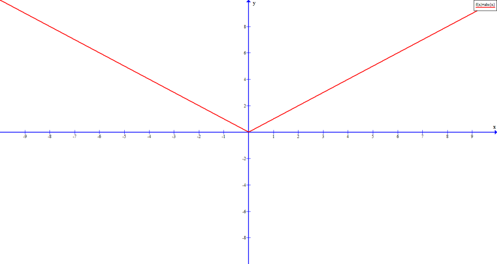
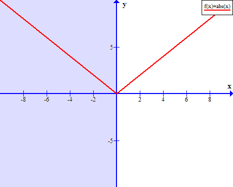
Consider the graph of absolute value function [latedpage] . This graph did not pass the horizontal line test and for each value, there exist two values.
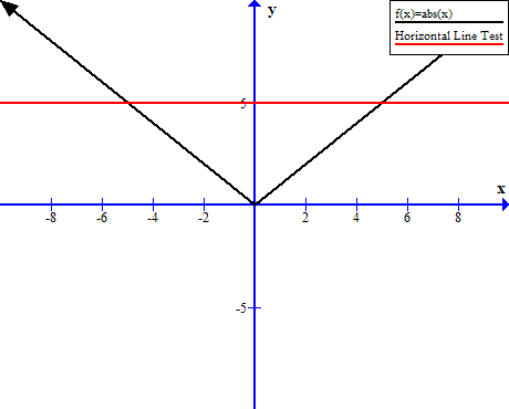
The graph will pass the horizontal line test if we restrict the domain to  , therefore, an inverse of absolute value function exists if we choose values between the interval
 ![[0, \infty]](https://notesformsc.org/wp-content/ql-cache/quicklatex.com-3767135a1b5e156f00be6ba3ee8ad08d_l3.png "Rendered by QuickLaTeX.com") .
.
The inverse of the new restricted absolute function is as follows.

We must observe two things,
- The absolute value cannot be a negative number, therefore,
 where
where  .
. - The function and its inverse does not reflect over
 , but
, but  .
.
 , but
, but  .
.