Functional Dependencies in DBMS: Use of FD in Table Design
A Functional dependency is used to describe the relationship between attributes of a relation. In other words, it explains how one or more columns of a database table determine other columns. In this article, we will discuss, the use of functional dependencies in table design and uses of functional dependencies.
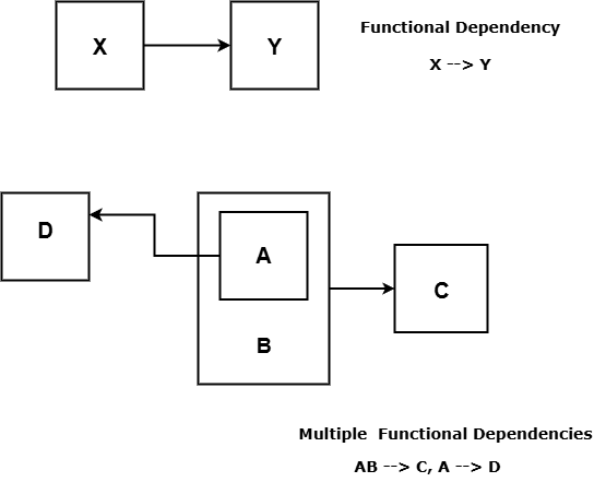
Let \Large X be a set of attributes, and \Large Y be another set of attributes.
If two rows of a relation have the same values for the attributes in \Large X, then they must have the same values for the attributes in \Large Y. This is known as the uniqueness property, and every functional dependency satisfies this property.
A functional dependency between \Large X and \Large Y is denoted as \Large X \rightarrow Y where \Large X is called the determinant and \Large Y is the dependent attribute set.
Example of Functional Dependency (FD)
Consider the following database table.
| StudentID | StudentName | Department |
|---|---|---|
| 20 | Peter Pan | Mathematics |
| 21 | Ravi Kumar | Physics |
| 22 | Kiran Joshi | Chemistry |
For each StudentID, there is only one StudentName. If two rows have same StudentID, then their StudentName must be same.
Similarly, for each StudentID there is exactly one Department. If two rows have same StudentID, then the deparment must contain same value.
This satisfies the uniqueness property of functional dependency.
Functional Dependencies in the Student Table
\Large StudentID \rightarrow StudentName\\StudentID \rightarrow Department
StudentName and Department are functionally dependent on StudentID. The StudentID is the determinant.
What Happens When There is no Functional Dependency
Consider another table with attributes – StudentID and CourseID.
| StudentID | CourseID |
|---|---|
| 21 | CS101 |
| 21 | CS102 |
| 22 | CS104 |
The table shows that some students are associated with more than one CourseID.
Therefore, StudentID does not uniquely determine CourseID, and the uniqueness property is not satisfied for this relationship.
This means the functional dependency
\Large StudentID \rightarrow CourseID
does not hold.
- StudentID does not uniquely determines CourseID.
- Student can be associated with many Courses.
A functional dependency exists only when the left-hand side attributes (determinants) uniquely determine the right-hand side attributes (dependent).
If one value of set \Large X, is mapped to multiple values of \Large Y, then \Large X \rightarrow Y is not functional dependency.
In the real world, a student can enroll in multiple courses. Although there is a meaningful relationship between students and courses, it is not a functional dependency.
While designing a database, the learner must carefully distinguish between:
- Meaningful relationships, and
- Functional dependencies, which require uniqueness.
Only relationships that satisfy the uniqueness property can be modeled as functional dependencies.
Composite Functional Dependency
Consider the following Grade Table.
| StudentID | CourseID | Grade |
|---|---|---|
| 21 | CS101 | A |
| 22 | CS104 | B |
| 23 | CS102 | B |
Step 1: Check for Individual Attributes
The StudentID alone cannot uniquely identify a student’s Grade. Students may obtain same grade for different courses.
Similarly, the CourseID alone cannot uniquely identify the grade of a student. Different student may get same grade for same course. There is no uniqueness.
Step 2: Check for Combination of Attributes
Consider the following combination:
\Large \{StudentID, CourseID\}Now we can uniquely identify a grade. Therefore, the functional dependency
\Large \{StudentID, CourseID\} \to Gradeholds.
This is called a composite functional dependency because the determinant consists of more than one attribute. In such a dependency, the left-hand side of the functional dependency is called a composite determinant.
Why Functional Dependencies Matter Before Normalization
Normalization is a formal process that restructures tables based on functional dependencies (FDs). Forms such as 2NF, 3NF, and BCNF are defined entirely in terms of FDs.
Therefore, normalization cannot begin until functional dependencies are identified and analyzed.
Role of Functional Dependencies (FDs)
Before normalization, functional dependencies are used to:
- Identify candidate keys
- Detect redundancy
- Explain insertion, update, and deletion anomalies
Each of these tasks relies on formal dependency rules, not intuition
Identifying Keys
Functional dependencies are used to find the candidate keys of a table. A candidate key is a set of attributes \Large K that determines all other attributes of the table, and no proper subset of \Large K can do the same.
To find candidate keys, we use a procedure called attribute closure.
The closure of attribute set \Large K written as \Large K^+
- is the set of all attributes
- that can be functionally determined from \Large K
- using the given functional dependencies.
The attribute closure of a set of attributes finds all attributes that are functionally determined by that set using the given functional dependencies. If the closure of a set K contains all attributes of the table and no proper subset of has this property, then is a candidate key.
Formally, if
- \Large K^+ contains all attributes of the relation.
- No other proper subset can this property,
\Large K is the candidate key.
Example – Find the Candidate key for Student Table.
Consider a Student table with four attributes: StudentID, CourseID, StudentName, and Grade.
We usually begin by computing the closure of single attributes.
\Large \{StudentID\}^+ = \{ StudentID\}The attribute itself is always included in its closure.
\Large StudentID \to StudentNameUsing the functional dependency StudentID → StudentName, we add StudentName to the closure.
\Large \{StudentID\}^+ = \{StudentID, StudentName\}StudentName is part of closure
\Large StudentID \to GradeThere is no functional dependency StudentID → Grade, so Grade cannot be added to the closure.
Let us check closure for CourseID.
\Large \{CourseID\}^+ = \{CourseID \}Initial value added to closure.
\Large CourseID \to GradeThe above is not a dependency.
\Large \{CourseID\}^+is not candidate set of keys.
Check closure of all attributes.
\Large \{StudentID, CourseID, Grade\}^+ = \{StudentID, CourseID, Grade\}Initial value added to closure.
This is the candidate key which functionally determine all attributes in the table.
Can we minimize it ?
Yes, the Grade can be determined by \Large \{StudentID, CourseID\}, but \Large StudentID or \Large CourseID cannot be determined alone.
Conclusion
The candidate key for the student table is the set \Large {StudentID, CourseID} because it determine all the attributes in the table.
\Large \{StudentID, CourseID\} \to Grade.
\Large\{StudentID, CourseID\} \to StudentID.
\Large \{StudentID, CourseID\} \to CourseID.
Another use of FD is to find the redundancy.
FD and Redundancy
From the above discussion, it clear that a functional dependency is either determinant or dependent in an optimized table. Any table attribute that it dependent on non-key attribute is likely to have duplicate values.
Therefore, functional dependencies reveal such attributes that are dependent on non-key attributes.
Consider the Student table with three attributes – StudentID, DepartmentID, and DeptName.
| StudentID | DepartmentID | DeptName |
|---|---|---|
| 20 | D101 | Mathematics |
| 21 | F102 | Physics |
| 22 | F102 | Physics |
The functional dependencies are:
\Large StudentID \to DepartmentID \\
DepartmentID \to DeptName
DeptName is not functionally dependent on StudentID.
The nature of functional dependency is Transitive.
\Large StudentID \to DepartmentID \to DeptName
We always want to remove the Transitive dependencies.
In these case, each student will not have exactly one value for Department name, but contains multiple redundant values.
Describe The Insert, Update and Deletion Anomalies
Here is a list of problems due to redundancies.
Insert anomalies – Unless student exists department id cannot be assigned , so a new department is not created if we don’t have a student. This is Insert anomalies.
Update anomalies – The table shows two students from same department – Physics. If we want to rename the Physics to something else, say Quantum Physics. We must change all the records where department name is Physics. This is update anomalies.
Deletion anomalies – If we delete the record for Student with id 20, then the department cease to exist. This is deletion anomalies.
Let us take another example.
The following Student table have four attributes – StudentID, CourseID, StudentName, and Grade.
| StudentID | CourseID | StudentName | Grade |
|---|---|---|---|
| 20 | M201 | Peter Pan | C |
| 20 | P101 | Peter Pan | A |
| 21 | X106 | Ravi Kumar | B |
| 21 | A44 | Ravi Kumar | A |
Let us identify the functional dependencies from the table.
\Large StudentID \to StudentName\\
\{StudentID, CourseID\} \to Grade
Clearly, the primary key is \Large \{StudentID, CourseID\}.
However, StudentName is only dependent on StudentID. This is Partial Dependency.
Conclusion
The solution to example 1 and example are same:
Example 1 – In case of transitive dependency, split the table into two.
| StudentID | DepartmentID |
|---|---|
| 21 | F102 |
| 22 | F102 |
| DepartmentID | DeptName |
|---|---|
| F102 | Physics |
| D101 | Mathematics |
The Student table has multiple same values, this is not redundancy. The StudentID is unique key and it identity the row in Student table uniquely.
The department table is totally unique because each department id has exactly one department.
Example 2 – In the case of partial dependency, you have to split the table again.
| StudentID | StudentName |
|---|---|
| 20 | Peter Pan |
| 21 | Ravi Kumar |
| StudentID | CourseID | Grade |
|---|---|---|
| 20 | M201 | C |
| 21 | A44 | A |
In the second example, StudentID or CourseID, alone cannot determine the Grade. Here are the functional dependencies from both tables.
Student Table
\Large StudentID \to StudentName
Grade Table
\Large \{StudentID, CourseID\} \to GradeThe separate tables ensure that each row is unique and do not have redundant data.
You have seen two different types of functional dependencies. In the next section, we shall explore all types of functional dependencies.
Types of Functional Dependencies (Using Tables)
The functional dependencies are classified based on attribute dependencies. Its the relationship between determinant attributes and dependent attributes.
Trivial Functional Dependency
A functional dependency \Large X \to Y from a set of attributes \Large X to a set of dependent attributes \Large Y is trivial if \Large Yis a subset of \Large X.
In other words, all the attributes of \Large Y are already in \Large X.
\Large X \to Y, is \hspace{4px} trivial \hspace{4px} if \hspace{4px} Y \subseteq XExample – Trivial Dependency
| StudentID | CourseID |
|---|---|
| 21 | A44 |
| 22 | P203 |
Observe that the key is \{StudentID, CourseID\} because StudentID or CourseID alone cannot be key.
Given the key, the following functional dependencies are Trivial.
\Large \{StudentID, CourseID\} \to StudentID\\
\{StudentID, CourseID\} \to CourseID
Axiom Used in Trivial Dependency
The Armstrong’s axiom used in trivial functional dependency is called the Reflexivity rule.
\Large FD: A \to A, \hspace{5px} because \hspace{5px} A \subseteq ANon-Trivial Functional Dependency
A functional dependency \Large X \to Yfrom a set of attributes \Large X to a set of dependent attribute \Large Y is Non-Trivial if \Large Y is non a subset of \Large X.
\Large X \to Y \hspace{4px} is \hspace{4px} Non-Trivial \hspace{5px} if \hspace{4px}Y \nsubseteq XExample – Non Trivial Dependency
| StudentID | StudentName |
|---|---|
| 20 | Peter Pan |
| 21 | Ravi Kumar |
The StudentID is the key and StudentName is dependent attribute. Also,
\Large StudentID \to StudentName,\\
\{StudentName\} \nsubseteq \{StudentID\}
The StudentName is not a subset or equal to set StudentID.
Axioms User in Non-Trivial Dependency
The non-trivial dependency is derived from other Armstrong’s axioms.
Suppose we have a functional dependency, \Large A \to \{B, C\} is called a Union Rule. The functional dependency can be decomposed into:
\Large FD: A \to \{B, C\} = \{A \to B\} \hspace{4px} and \hspace{5px} \{A \to C\}Completely Non-Trivial Functional Dependency
A functional dependency \Large ( X \to Y ) is a completely non-trivial dependency for two sets of attributes \Large X and \Large Y if:
\Large X \cap Y = \empty
In a completely non-trivial dependency, the sets \Large X and \Large Y are disjoint, and their intersection is a null or empty set.
Example – Completely Non-Trivial Dependency
| StudentID | DeptName |
|---|---|
| 20 | Mathematics |
| 21 | Physics |
| 21 | Computer Science |
Notes that \Large StudentID \cup DeptName are disjoint sets.
However, the functional dependency holds.
\Large StudentID \to DeptName
The functional dependency is correct, but each student can have more than one department. The student with ID 21 has two separate departments. This will cause redundancy in the table. You must normalize the table in such cases.
Full Functional Dependency
A dependency from \Large X \to Y is Full dependency if:
- \Large Y is dependent on all attributes of \Large X.
- No proper subset of \Large Xcan determine \Large Y.
Symbolically,
\Large \begin{aligned}
&X \to Y \hspace{5px} is  \hspace{5px} a \hspace{5px} Full \hspace{5px}Functional \hspace{5px} Dependency \hspace{5px} if:\\
&1. \hspace{3px}Y \not \subset X\\
&2. \hspace{3px} X' \not \to Y, \hspace{5px} where \hspace{5px} X' \subset X
\end{aligned}
Example – Full Functional Dependency
In this example, consider Student table with StudentID, CourseID and Grade.
| StudentID | CourseID | Grade |
|---|---|---|
| 20 | M203 | C |
| 21 | A44 | A |
This is a full functional dependency where Grade is dependent on key \Large \{StudentID, CourseID\}.
\Large \{StudentID, CourseID\} \to GradeNow to validate, that this is full functional dependecy, we must check the conditions.
- \Large Y is not a subset of \Large X.
\Large \{StudentID, CourseID\} \nsubseteq Grade2. \Large X' cannot determine \Large Y, where \Large X' is proper subsets of \Large X.
\Large StudentID \not \to Grade\\
CourseID \not \to Grade
Hence, it is proved that the functional dependency is a full functional dependency.
Partial Functional Dependency
A functional dependency \Large X \to Y is a Partial functional dependency if:
- \Large X is composite. In other words, \Large X has more than one attributes.
- \Large Y depends only on part of \Large X.
Example – Partial Functional Dependency
Consider the student table.
| StudentID | CourseID | StudentName |
|---|---|---|
| 20 | CS101 | Peter Pan |
| 21 | A44 | Ravi Kumar |
We have two functional dependencies in the above table.
\Large \{StudentID, CourseID\} \to StudentName\\
StudentID \to StudentName
Let us check the conditions for partial dependency.
- \Large X is composite. This condition is true because \Large \{StudentID, CourseID\} uniquely determine all the attributes in the student table.
- \Large Y depends on part of \Large X. This is also true, because StudentName is dependent only on StudentID, and not on CourseID of composite key \Large \{StudentID, CourseID\}.
The partial dependency causes redundancy and violates the second normal form \Large (2NF). You will learn \Large (2NF) in future posts.
Transitive Functional Dependency
A functional dependency \Large X \to Y is Transitive if there exists another dependency \Large Y \to Z such that \Large X \to Z also exists. The \Large X \to Z is also a function dependency.
\Large \to Y \hspace{5px} is \hspace{5px} Transitive \hspace{5px} if:\\

X \to Y \hspace{5px} and \hspace{5px} Y \to Z \hspace{5px} implies \hspace{5px} X \to Z
Example – Transitive Functional Dependency
Consider the following Employee table.
| EmployeeID | DeptID | DeptAddress |
|---|---|---|
| 4331 | D12 | New Delhi |
| 4332 | D13 | Chennai |
| 4333 | D14 | Mumbai |
| 4334 | D14 | Mumbai |
We see two functional dependencies in the Employee table.
\Large EmployeeID \to DeptID\\
DeptID \to DeptAddress
Since, EmployeeID determines DeptID and DeptID determines DeptAddress.
A transitive functional dependency. exists between ExployeeID and DeptAddress.
\Large ExployeeID \to DeptAddress
A transitive dependency contains redundant data.
If you look at the Employee table, the department address Mumbai is repeated every time when an employee has department ID of D14. In these cases, splitting the table is the best solution.
Now, you know everything about Functional dependencies, let us summarize what you learned.
Summary
These are important points to remember for exams.
Uses Of Functional Dependencies (Concept Overview for Revision)
| Purpose of FDs | Explanation |
|---|---|
| Identify Keys | Determine candidate keys and primary keys using attribute closure. |
| Detect Redundancy | Reveal the duplicate storage of same information across many rows. |
| Explain Anomalies | Identify Insertion, Update and Deletion anomalies. |
| Guide the Normalization Process | Decompose relations into normal forms. |
| Improve Table Design | Ensure minimum duplicates and improve logical data organizations. |
Types of Functional Dependencies
| Dependency Type | Concept |
|---|---|
| Trivial Functional Dependency | Dependent attribute is already part of Determining attributes. |
| Non-Trivial Functional Dependency | Dependent attribute is NOT part of Determining attributes. |
| Completely Non-Trivial Functional Dependency | Dependent and Determinant attributes have nothing in common. |
| Full Functional Dependency | The Dependent attributes depend on the entire set of Determining attributes and not on any proper subset of Determining attributes. |
| Partial Functional Dependency | Depending attributes depends only on subset of Determining Attributes. |
| Transitive Functional Dependencies | Dependent attributes indirectly dependent on the Determining attributes. |
Data Models in DBMS: Data Abstraction, Levels, and Types
Data models are fundamental concepts in DBMS that help in database design. They enable communication between database designers, application developers, and end-users.
A Data model defines how data is structured, organized, and represented in a database system. The topic is foundation for database design, and it is an important part of the DBMS syllabus.
In this post, we will explain the concepts of data models, data model levels, and understand different types of data models. This topic is frequently asked in university examinations and competitive examinations like GATE, etc.
Before we begin, let’s understand data abstraction.
What is Data Abstraction?
The data abstraction means only exposing the essential data to the users and hiding the implementation details. We don’t show the storage details.
The purpose of data abstraction is:
- Provide security and data protection.
- Data independence
- Reduce complexity
- Easy maintenance
Provide security and data protection
The data abstraction keeps different access for different users. It hides the sensitive data from normal users. Users cannot access the data directly without authentication.
Data Independence
Data abstraction is independent of physical storage. A change in storage structure such as files, indexes, etc., will not affect the application level data. They are independent of each other.
Reduce Complexity
Keeping separate layers of data and hiding their implementation details reduces complexity. Users only see what is necessary for them.
For example, users interact with logical tables, without knowing the storage details.
Easy Maintenance
We already mentioned that data abstraction is data independence. Each layer is separate and does not affect the higher layer. We can repair physical disks, without affecting user’s access to tables.
This makes the maintenance process easy.
What is Data Model ?
The data model is the blueprint that defines the structure of the database. It is the foundation of database design. The structure of the database includes its
- Data types
- Relationships and
- Database constraints.
The data model is designed and organized to solve the data requirements of a specific application or specific domain, not all applications. It only supports a specific problem area.
A key feature of a data model is the data organization, which defines how data and relationships are structured in the database.4
In next section, you will learn more about different levels of data models.
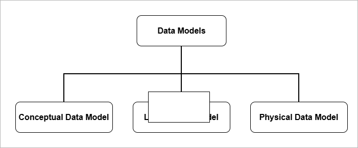
Three Levels of Data Models
It is necessary to separate the data models into three distinct levels of modeling. Each level of data model collects different data and implements them differently.
- Conceptual Data Model
- Logical Data Model
- Physical Data Model
Conceptual Data Model
A conceptual data model is a high-level model that provides
- an overall logical view of the database that is easy for non-technical stakeholders to understand. It consists of real-world concepts and business logic.
- It tells us what kind of data is required, independent of database or storage details. It reveals business requirements such as entities and their relationships.
- The conceptual layer enables communication between the database designer, application developer, and end users. All of them collaborate to build a database system that solves a specific problem.
- The conceptual level serves as a blueprint for both the logical data model and the physical data model.
In relational database systems, conceptual modeling involves creating an Entity–Relationship (E–R) model or an object model. Its main purpose is to answer two questions:
- What data is required?
- How should the data be organized ?
At the conceptual data model level, data is represented as entities and their relationships, where an entity represents a real-world object.
Object modeling uses UML (Unified Modeling Language), use-case diagrams, etc., to model user interaction with the database through a software system.
After conceptual data model is completed, the next step is to design a logical data model.
Logical Data Model
The main purpose of logical data model is to answer one question, “How is the data organized?”.
The logical data model is used to design database relations and their relationships based on the conceptual model, without specifying physical storage details.
The logical (relational) model is the core of database systems (DBMS) because it defines how data is organized, related, and accessed.
The E–R diagram from the conceptual model is translated into a relational model.
Data is organized into tables (relations) that contain columns (attributes), keys, and relationships.
The next step after the logical data model is to implement the database on disks and storage devices
Physical Data Model
The physical data model defines the files, storage structures, and other storage-level details of the database. This level answers the question:
“How is the data stored?”
The physical data model includes:
- File system
- Indexes
- Storage allocation
- Records placements
- Access paths
The storage level details are hidden from the common users of the database system.
- At storage level, faster searches is achieved through indexes,
- Disk performance is enhanced using disk access algorithms.
- Storage security ensures protection of servers from damage, power failures, and theft.
Different types of models correspond to different levels of data modeling. The conceptual level captures concepts in the form of entities and relationships. The logical level defines how data is organized. The physical level selects efficient storage structures.
In the next section, we discuss different types of data models.
Types of Data Models (Logical)
Logical models represent different ways of organizing data and relationships. The main types are:
- Hierarchical model
- Network model
- Relational model
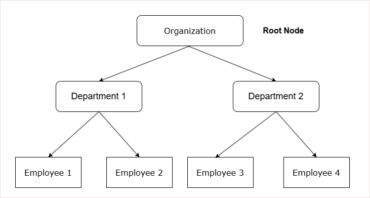
Hierarchical Data Model
The hierarchical data model stores data in a tree-based structure.
- The tree-like structure helps represent natural hierarchies.
- A strict parent–child relationship ensures data integrity.
- The tree-based structure is simple and predictable.
- The data retrieval is faster if you know the path as it is fixed.
- Access begins from the root node, which means nodes closer to the root are accessed more quickly.
Components of a Hierarchical Data Model
1. Tree Structure
The hierarchical data model is based on a parent–child relationship.
- Each parent can contain multiple child nodes.
- Each child node can have only one parent.
2. Nodes
Data is organized into a logical units called nodes.
- Each node represents a specific type of record.
3. Root Node
The top of the tree contains a single node called the root node.
- The root node has no parent.
- It is the starting point for data access and navigation.
4. Leaf Nodes
The lowest-level nodes in the tree are called leaf nodes.
- A leaf node has no children.
* Data organization begins from the root node.
* It follows strict parent–child relationships.
* Each child has only one parent, while each parent can have multiple children.
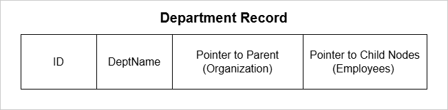
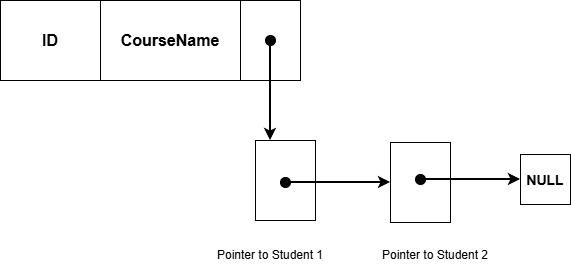
How records are stored in Hierarchical model?
The records in hierarchical model has many fields, including the following;
- A pointer to parent node, except root node.
- Pointers to many child nodes
Data retrieval in a hierarchical data model requires traversing the nodes from the root node to the specific record.
- You can only traverse records starting from the root node.
- Retrieval is top-down and one-way.
In a hierarchical data model, data retrieval is one-way, typically from parent to child, following a fixed top-down path.
Limitations of Hierarchical Model
The hierarchical data model has several limitations:
- The structure is rigid and suitable only for one-to-one or one-to-many parent-to-child relationships.
- The search path is fixed and always begins from the root node.
- There is no support for many-to-many relationships.
An improved alternative to the hierarchical model is the network model.
In the next section, you will learn about the network model.
Network Data Model
The network data model has a graph-like structure.
- There is no root node, unlike the hierarchical model.
- In this model, a child node can have multiple parents, and a parent can have multiple children.
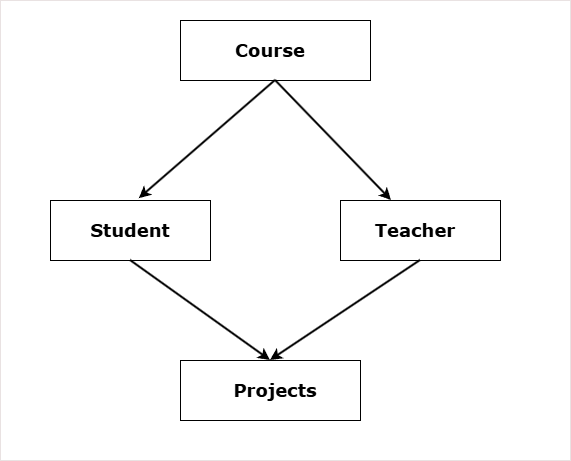
The diagram shows a network data model for school where:
- One course has one or many students.
- One course has one or many teachers.
- One student has one or more projects to complete.
- One teacher guide students on one or many projects.
Components of Network Data Model
The main components of network data model are:
- Record Type
- Data Item (attribute)
- Set Type
- Owner Records
- Member Records
- Links (Pointers)
Record Type
The record type define the structure of the record. It is similar to concept of relational schema in RBDMS. It defines three things:
- Attribute or field names
- Data types of the fields
- Format of the data such as dates, integer, double, etc.
Examples:
Student (ID, Name, Course);

Course (ID, Name, Details);
Each instance of the record type is called record occurance.
Data Item
Data item is an attribute inside a record. Each record is made of many data items.
Example:
Car record have model, color, price data items.Set Type
The set type is the most important component. It define the relationship between two record types. It has:
- Owner record type
- Member record type
Example:
SET Enrollment
Owner : Course
Member: Students
One Course can have many students as members. One student can have many such owners. This is the reason, the network data model is a graph, not a tree.
Owner Records
The record type that is an owner of the set. There are two rules for owner records follow:
- Only one owner for a set.
- An owner can have multiple members.
When set is defined there are EXACTLY two record types defined;
- An Owner record type
- A Member record type
An owner record can be member of another set.
A member record type is one, but there are many member record occurrence for a single owner record occurrence.
Benefit over Hierarchical Data Model
The benefit of network model over hierarchical data model is relationships. The network model supports following types of relationships.
- One-to-One (1:1)
- One-to-Many (1:N)
- Many-to-Many (M:N)
The improvement is the many-to-many relationships using sets.
If one set is Courses – to – Students (1: N), then another set from Students-to-Course (1:N) will create a many-to-many relationship. This is better then rigid hierarchical data model.
Limitations of Network Data Model
The network model is definitely an improvement over the hierarchical data model. However, it has its own limitations.
- Complex Structure – Network model stores relationships and records with the help of links and pointers. This add complexity to the structure.
- Complex way to Insertion, Updation, and Deletion of Records – An insertion, update, or deletion of record requires changing many links and pointers. Programmers manually maintain such complex structure. After a deletion, lot of links must be re-adjusted properly.
- No Data Independence – There is not data independence because if data links and pointers change, the application code must also change.
- Data Corruption – Missing link or pointers can corrupt data.
- Less Abstraction – It is very close to how data is stored, not as abstracted as Relational model.
The relational data model or RDBMS is much more reliable and flexible that the network model. You will learn about relational model throughout the DBMS course on our site.
Relational Data Model
The relational data model is the most popular data model at the time of writing.
At the conceptual level, the relational model uses the Entity–Relationship (E–R) model to capture the business model or business logic.
In other words, the E–R model serves as the conceptual-level blueprint from which a relational data model can be created.
The relational model stores data in the form of a table or relation.
Relation – A relation is an abstract, unordered collection of data with no duplicate records.
- Each attribute has a data type that specifies the kind of values it can hold.
- It is a set of tuples (rows).
- Attributes (columns) define the properties of a real-world object or entity.
Table – A table is the physical implementation of a relation.
- The records in a table are ordered in the database using an index.
- It consists of rows and columns.
- Unlike a relation, a table can allow duplicate records.
Entity – A single real world object represented as one row or a tuple is called an entity.
For example,
Student( id, name, age); is relation.
(100, "Raju", 23) is an entity.
Entity Set – A set of entities is called entity set and it shares common attributes and represented by relation or table. Entity set is similar entities with different data values for same attributes.
The database items in relational model are records. A set of records with similar attributes are called relations or tables.
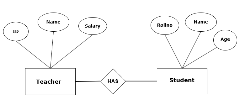
The above E-R model shows a conceptual school database with two entity sets – Teacher and Student.
The data is stored as tables with rows and columns in the database.
For example,


Relationships in Relational Model
Compared to hierarchical model and the network model, the relational model is more flexible. Yet, it employs data abstraction at all levels and provide data integrity and security.
The relationships in relational model is supported by cardinality ( number of entities in the relation). It supports following models:
- One-to-One (1:1)
- One-to-Many (1:N)
- Many-to-One (N:1)
- Many-to-Many (N:M)
Advantages of Relational Model
The relational model has many advantages.
- Simplicity – It is simple to use. The storage is in the form of table with rows and columns.
- Data Integrity – Each table has constraints such primary keys, and rules for attributes which maintain high accuracy in storing data.
- Data independence – Each level of this model is independent of high levels.
- Transactions are ACID compliant – Each transaction either complete successfully or fail and do nothing. The follow ACID properties – Atomicity, Consistency, Isolation, and Durability.
- Flexibility – Unlike Hierarchical model, or Network model, we can easily update tables and records.
- SQL – Relational model provides special query language to retrieve information from the database.
In future posts, you will only learn about Relational data model.
Summary
Data model is about how data is structured, organized, and represented in database systems. There are three levels of data model.
- Conceptual
- Logical
- Physical
There are different types of logical models in database system. The three main types are:
- Hierarchical model – Stores data as a tree based structure.
- Network model – stores data as a graph-like structure.
- Relational model – stores data in tables with rows and columns.
Relational Model and Algebra
Relational Model and Algebra
Entity-Relationship Modeling (E-R Modeling)
Entity-Relationship Modeling (E-R Modeling)
DBMS Introduction and Architecture
DBMS Introduction and Architecture
SQL Basics Explained: Commands, Queries, and Examples
SQL (Structured Query Language) is the standard query language for databases. It is not just for querying data, but a complete language used to control, manage, and maintain a relational database system.
Why only RDBMS (Relational Database Management Systems)?
Because NoSQL systems such as MongoDB, CouchDB, and others use different storage structures like JSON, BSON, or document-like formats. They do not follow the relational model, so SQL is not used in the same way.
This post will explain basic SQL commands and queries with examples. It will help you get started with your SQL journey.
Types of SQL Commands
The different types of SQL commands are categorized based on their functions within the database system. These commands can define database structures such as tables and indexes, insert or update data, delete values from tables, retrieve information through queries, control user access, and manage transactions.
A list of SQL command categories is given below:
- Data Definition Language (DDL)
- Data Manipulation Language (DML)
- Data Query Language (DQL)
- Data Control Language (DCL)
- Transaction Control Language (TCL)
Let’s discuss each of them in detail.
Data Definition Language (DDL commands)
Data Definition Language (DDL) consists of SQL commands used to create, modify, and delete database structures such as databases, tables, views, and indexes. All DDL commands are auto-committed, meaning the changes take effect immediately and permanently, and cannot be rolled back.
Common DDL commands are listed below.
- CREATE
- ALTER
- DROP
- TRUNCATE
- RENAME
CREATE Command
The CREATE command is used to create database objects like databases, tables, indexes, and views.
Examples of CREATE
1. To create a database.
CREATE DATABASE library;2. Command to create a table.
CREATE TABLE books (
    book_id INT AUTO_INCREMENT PRIMARY KEY,
    title VARCHAR(200) NOT NULL,
    author VARCHAR(150),
    publisher VARCHAR(150),
    published_year INT,
    price DECIMAL(10,2)
);
Note: If you are running SQL commands on MySQL , then make sure run to USE <database name>;
before any SQL command. Otherwise , it won’t work.
3. Command to create views.
A view is a virtual table based on SELECT query.
CREATE VIEW cheap_books AS
SELECT title, author, price
FROM books
WHERE price < 300;
4. Command to create a unique index.
A database index helps in faster searches.
CREATE UNIQUE INDEX idx_isbn
ON books(isbn);
ALTER Command
The ALTER command can modify the structure of an existing database object. It allows you to change, add and delete columns, constraints, and any other properties without deleting the table or its data.
The ALTER command is mostly used for:
- Add a new column
- Modify the data type of an existing column
- Rename a column
- Drop (remove) a column
- Add or remove constraints
- Rename the table
Examples of ALTER Commands
1. Add a New Column to Existing Table.
If you are using My SQL, make sure to run USE <database name>; before any other SQL commands, otherwise, it won’t work.
ALTER TABLE books
ADD isbn VARCHAR(30);
2. Modify the data type of an existing column
ALTER TABLE books
MODIFY price DECIMAL(12,2);
The initial data type of the price attribute was DECIMAL (10, 2);. The new data type is DECIMAL(12, 2);.
3. Rename a Column
ALTER TABLE books RENAME COLUMN title TO book_title;The RENAME takes two parameters:
- Old column name
- New column name
4. Drop a Column
ALTER TABLE books
DROP COLUMN published_year;
This will remove the column published_year from the table. Any data for the column is permanently deleted, including constraints, indexes, etc.
How to know if the column is deleted ? Use DESCRIBE books; or SHOW COLUMNS FROM books;
You should see all columns except published_year.
5. Add or Remove a Constraint
ALTER TABLE books
ADD CONSTRAINT unique_title_author UNIQUE (title, author);
The command above will add a UNIQUE constraint on the title and author columns. All combination of title and author are unique.
How do we know if the constraint was added?
The command SHOW INDEX FROM book; will return non_unique = 0 which means that all entries are unique.
6. Rename the table
ALTER TABLE books RENAME TO library_books;DROP Command
The DROP command helps to delete database objects. You can delete databases itself using the DROP command. This command is auto-committed meaning the action cannot be undone, and deletion is permanent.
You can delete following using this command.
- Database
- Table
- Views
- Index
- Columns via ALTER TABLE command
- Constraints via ALTER TABLE command.
Examples of DROP Command
We can see example of first 4 objects from the above list. For examples of drop column and constraints, refer to the ALTER command examples.
Before running any command in My SQL , run following command, USE <database name>;.
1. Remove a Database
DROP DATABASE members;2. Remove a Table
DROP DATABASE memberships;3. Remove Views
DROP VIEW cs_books;4. Remove index
DROP INDEX idx_isbn ON Library;TRUNCATE Command
This command deletes all the rows from a table but keep the schema and structure of intact. It is more efficient than DROP command which delete the entire object.
The TRUNCATE command cannot be used for deleting specific roles.
Example of TRUNCATE command
If the books table is empty, insert the following records, otherwise, skip this step.
INSERT INTO books (book_id, title, author, price) VALUES (12, 'Ashtavakra Geeta', 'Ashtavakra', 120.43);
INSERT INTO books (book_id, title, author, price) VALUES (13, 'Sri Ramayanam', 'Maharshi Valmiki', 550.50);
INSERT INTO books (book_id, title, author, price) VALUES (14, 'Sri Mahabharatam', 'Maharshi Vedvyas', 1000.35);
Now run the truncate command.
TRUNCATE books;To know the effect of TRUNCATE command, run the following SQL command. This command will try to retrieve all the records from book table.
SELECT * FROM books;If you only see a structure of table in the results, but no records. The TRUNCATE has been successful. The TRUNCATE command will remove all records.
RENAME Command
The RENAME command will help us rename the TABLE. There are two ways to achieve this goal.
- Rename the Table directly.
- Use the ALTER TtBLE command.
Examples of RENAME Command
1. Direct renaming.
RENAME TABLE books TO library_books;2. Using ALTER TABLE Command.
ALTER TABLE books RENAME TO library_books;DML Commands
Data Manipulation Language (DML) commands are those commands that work with actual data records stored inside database tables. They are used to insert, modify, retrieve and delete the records.
Why are DML commands used:
- Add a new record
- Modify an existing record.
- Retrieve and display existing records.
- Delete records from one or more tables.
List of DML commands
There are many DML commands, the most common ones are listed below.
- INSERT
- UPDATE
- SELECT
- DELETE
Let’s discuss each of them briefly.
SQL questions in university exams are usually application-based. Regular practice of basic queries (SELECT, WHERE, JOIN) helps in answering 2–5 mark SQL questions accurately.
INSERT Command
This command simply inserts a new record into the table with the values you provide. The table name and the data values must be correct for insert to work.
Before you try this command in MySQL, do the following.
CREATE DATABASE university;
USE university;
To insert values into the University database, create a table for Students and insert values.
CREATE TABLE students (
    student_id INT PRIMARY KEY,
    first_name VARCHAR(50),
    last_name VARCHAR(50),
    age INT,
    email VARCHAR(100),
    course VARCHAR(100)
);
Now, insert values using the INSERT command.
INSERT INTO students (student_id, first_name,last_name, age, email, course)
VALUES (1, 'Rakesh', 'Kumar', 20, '[email protected]', 'Physics');

INSERT INTO students (student_id, first_name,last_name, age, email, course)
VALUES (2, 'Karuna', 'Nair', 20, '[email protected]', 'Mathematics');
UPDATE Command
This command will update records in a table.
We have entered the wrong age for student ‘Karuna’, which we now want to change.
UPDATE students
SET age = 25
WHERE student_id = 2;
SELECT Command
This command helps query the database, retrieve results and displaying them. You can query the database based on conditions.
For example, to view the updated information of student “Karuna”, run the following command.
SELECT * FROM students WHERE student_id = 2;The following command will retrieve records from entire table.
The asterisk (*) selects all columns from the table. The WHERE clause is used to filter rows based on conditions.
SELECT * FROM books;DELETE Command
This command helps delete the records from a table in a database.
DELETE FROM students
WHERE id = 1;
Data Query Language (DQL)
The Data Query Language (DQL) is used to retrieve data from the database based on specific conditions. It does not modify or change table values. — It only reads data.
SELECT is the only command to run query. But DQL can do lot of things such as:
- Retrieve data from one or more tables.
- Filter and extract data based on conditions.
- Sort data in ascending or descending order.
- Group data.
- Join multiple tables.
Examples of DQL Commands
Here are some examples of different tasks carried out using SELECT command.
1. Get all the records from a table.
SELECT * FROM students;2. Filter and get results based on conditions.
SELECT first_name, age FROM students;This time the query return only the first name and age column from the students table.
3. Sort the results.
You can sort the query results by using ‘ORDER BY’ clause.
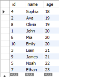
Ascending order
SELECT * FROM students
ORDER BY age ASC;Result:
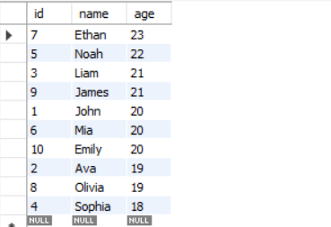
Descending order
SELECT * FROM students
ORDER BY age DESC;Result:
4. Group the results
GROUP BY is used to organize rows that share identical values in one or more columns. It is commonly used together with aggregate functions such as COUNT(), SUM(), or AVG() to summarize data.
Aggregate functions are take multiple of rows data and return a single summarized value. Use these functions to calculate total, averages, or maximum /minimum values.
- SUM()
- COUNT ()
- AVG()
- MAX()
- MIN()
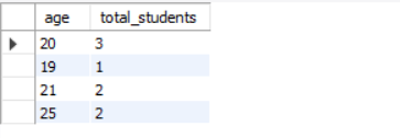
Grouping students on age and counting students for each group
SELECT age, COUNT(*) AS total_students
FROM student
GROUP BY age;
The SQL command does two things.
- Group all students in groups where age is same.
- Count the total number of students for each group.
Result:
5. JOIN two or more tables
The JOIN command joins two or more tables based on one or more shared shared columns. All types of joins use a shared column except
- CROSS JOIN
- SELF JOIN
What are different types of JOINs?
Here is a list of common joins.
- INNER JOIN – When all records from both table are matching.
- LEFT JOIN – All records of left table and matching records from right table.
- RIGHT JOIN – All records of right table and matching records from left table.
- FULL JOIN – All records from both tables.
- CROSS JOIN – Return all combination of both tables ( A Cartesian Product).
- SELF JOIN – A Join on itself ( A reflexive relationship).
JOIN Command Examples
We shall see examples of JOIN now.
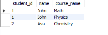
INNER JOIN
SELECT
    s.student_id,
    s.name,
    c.course_name
FROM students s
INNER JOIN courses c
ON s.student_id = c.student_id;Result:
Return records of all students who have joined a course.
LEFT JOIN
SELECT
    s.student_id,
    s.name,
    c.course_name
FROM student s
LEFT JOIN course c
ON s.student_id = c.student_id;Result:
The LEFT JOIN returns all entries from left table (student) and those entries from course table where student.student_id matches course.student_id.
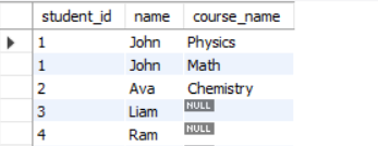
All non-matching entries will have a Null value.
RIGHT JOIN
SELECT
    s.student_id,
    s.name,
    c.course_name
FROM student s
RIGHT JOIN course c
ON s.student_id = c.student_id;Result:
The RIGHT JOIN returns all entries from right-hand table(course) and matching records from student table. Non-matching entries will have a Null value.
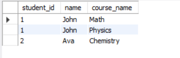
Note that there is no Null in the output, because there are no mismatched records. Every course has a student.
FULL JOIN
SELECT
    s.student_id,
    s.name,
    c.course_name
FROM
    student AS s
LEFT JOIN
    course AS c
ON s.student_id = c.student_id

UNION

SELECT
    s.student_id,
    s.name,
    c.course_name
FROM
    student AS s
RIGHT JOIN
    course AS c
ON s.student_id = c.student_id;
MySQL do not support FULL JOIN, therefore, you can use UNION command to include results from LEFT JOIN and a RIGHT JOIN.
The FULL JOIN returns all rows from both tables – student and course. If records match, it shows the matching data, if not, the missing values are filled with Null.
Result:
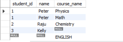
The result shows all matching records from student and course table. It also includes all records that do not match and fill the empty column with Null.
The student ‘Kelly’ did not join any course and the course ‘ENGLISH’ has no students.
CROSS JOIN (Cartesian Product)
SELECT
    student.student_name,
    course.course_name
FROM
    student
CROSS JOIN course;Result:
The CROSS JOIN produces a Cartesian product of two tables. Every row of first table is paired with every row of second table.

Data Control Language (DCL)
The Data Control Language (DCL) in SQL consists of commands that manage access control, permissions, and data security. It decides who can do what.
It has three main tasks:
- Grant permission to users.
- Revoke the permission given to users.
- Secure the data and make sure authorized access.
DCL Commands
There are only two commands. Different version of SQL uses slightly different syntex, but they mean the same thing.
- GRANT
- REVOKE
For example, MySQL doesn’t use DENY, but SQL Server does. MySQL uses REVOKE statements.
Examples of DCL Commands
Grant permission to SELECT, INSERT to the user ‘Kiran’ using GRANT command.
GRANT SELECT, INSERT ON students TO 'kiran'@'localhost';Revoke all permissions for user ‘Kiran’ using REVOKE command.
REVOKE ALL PRIVILEGES, GRANT OPTION FROM 'kiran'@'localhost';Transaction Control Language (TCL)
A transaction is a group of SQL commands executed as one unit of work. Either all of the operations succeed or fall fails.
Transaction Control Language (TCL) controls these operations which are nothing but several DML statements such as INSERT, UPDATE, and DELETE.
TCL Commands
The Main TCL Commands are:
- COMMIT
- ROLLBACK
- SAVEPOINT
- SET TRANSACTION
Examples of TCL Commands
COMMIT
When transaction is successful. The Commit command save the changes to the database permanently.
START TRANSACTION;

UPDATE accounts SET balance = balance - 500 WHERE id = 1;
UPDATE accounts SET balance = balance + 500 WHERE id = 2;

COMMIT;
In the example above, both succeed or both fails.
Learn more about Database Transaction States.
Want to get in-depth knowledge on Transaction Processing?
Visit Transaction Processing in DBMS: Concept, Properties and Examples.
ROLLBACK
When the transaction fails, database can become inconsistent and all changes are ROLLBACK to bring the database into a consistent state.
START TRANSACTION;
DELETE FROM student WHERE student_id = 4;
ROLLBACK;  -- Undo the delete
SAVEPOINT
The SAVEPOINT creates a checkpoint, so that we can partially rollback to it, if necessary.
START TRANSACTION;
UPDATE products SET price = price + 10;
SAVEPOINT p1;
UPDATE products SET price = price + 5;
ROLLBACK TO p1;   -- Undo only the second update
COMMIT;
You can understand the example, by knowing what each step does.
- Transaction starts.
- product price is set to price + 10;
- We created a SAVEPOINT, if anything goes wrong, go back to SAVEPOINT.
- The product price is incremented by 5. This is an unwanted activity.
- Rollback to the nearest correct price and state.
- Commit the changes if all operations are completed successfully.
SET TRANSACTION
The SET TRANSACTION define the properties of a transaction. A set transaction changes following properties:
- Isolation Level – Isolation is one of the ACID properties that controls how a transaction must behave during concurrent access. Therefore, isolation level decides how much the current transaction must “see” from other transactions, running simultaneously.
- Read/Write Mode – It defines whether transaction can (read and write) or (read only).
- Scope – This property decides whether settings are applied to Next transaction or Current Transaction only.
SET TRANSACTION READ ONLY;

START TRANSACTION;

SELECT * FROM products;  -- Allowed
UPDATE products SET price = 100;  -- Not allowed

COMMIT;
Summary of SQL Basic
| Category | Full Form | Purpose | Commands |
| DDL | Data Definition Language | Create or Modify database structures. | CREATE, ALTER, DROP, TRUNCATE, RENAME |
| DML | Data Manipulation Language | Manage data inside tables. | INSERT, UPDATE, DELETE |
| DQL | Data Query Language | Get data from Tables. | SELECT |
| DCL | Data Control Language | Control user access and permissions. | GRANT, REVOKE |
| TCL | Transaction Control Language | Manage transactions. | COMMIT, ROLLBACK, SAVEPOINT, SET TRANSACTION |
If you are starting with SQL and preparing for exams, structured practice is essential. The free SQL Starter Kit includes:
- SQL Basics Explained (PDF) – clear explanations with examples
- MySQL Installation Guide – step-by-step setup for practice
- SQL Practice Sheet – exam-relevant questions with queries
Functional Dependencies in DBMS: An In-Depth Guide
Functional dependency is a key concept in database design. When designing database relations, it is important to avoid situations that cause update anomalies—problems that occur when changes to data are not properly reflected across all related records. If copies of a relation are not updated consistently, the database can become inconsistent or corrupt.
Another common issue is redundant data. Storing the same information multiple times makes the database complex and increases the risk of update anomalies. Omissions or accidental deletions can also lead to anomalies.
Functional dependencies help in designing robust databases by providing tools such as FD closure, attribute closure, and canonical cover.
These concepts form the foundation for normalization, a process that organizes database relations to reduce redundancy and improve consistency. Normalization is a separate topic, so in this guide, we focus exclusively on understanding functional dependencies in depth.
What is Functional Dependency?
A functional dependency (FD) is a relationship between two sets of attributes in a relation (table). It shows how one set of attributes determines another. A functional dependency is key to designing a relation in database design. The main task of functional dependency is to remove update anomalies.
Before we define a functional dependency , you must understand the difference between the term – relation and table.
Key difference between Relation and Table
| Key Aspect | Relation | Table |
| Definition | Relation is a mathematical and abstract concept from relational theory. | Table is a physical structure that store data in rows and columns. |
| Order of Rows | The rows or tuples have no specific order | The rows have order in storage and retrieval by default. Then ordered if Order By clause is used. |
| Duplicate Rows | No duplicate row – all rows are unique. | Allows duplicate unless Primary key is set to make every row unique. |
| Attribute Names | Must be unique | Must be unique, but aliasing is possible. |
| Null Values | Not part of relational model. | Allowed in table to represent empty or unknown data. |
| Implementation | Rules defined in relational algebra and theory | Use RDBMS softwares like MySQL, Oracle, etc. |
| Schema | Define attributes and domain types | Define the attributes and their data types |
Note that Relation is a mathematical concept that defines the construction of logical structure of tables.
Formal Definition of Functional Dependency
The formal definition of functional dependency, also known as FD is as follows.
“If there is relation schema R with random subset X and Y such that an instance r of R satisfy functional dependency,
FD: X \rightarrow Y
this means for any two tuples t_1 and t_2 in r.
if \space t_1[x] = t_2[x], then \space t_1[y] = t_2[y]
which means Y is functionally dependent on X. In other words, FD: X \rightarrow Y satisfy “uniqueness property”. Every x uniquely determine the value of y.
Determinant and Dependent
In a functional dependency X \rightarrow Y, X is called Determinant and Y is called the Dependent.
Sometimes, an functional dependency does not hold for a relation schema R because the uniqueness property is violated – that is, multiple y values for the same x. Such FDs can be discarded.
The Set of Functional Dependencies
A set of functional dependencies (FDs) is a collection of one or more functional dependencies defined on a relation R.
If relation schema R has attributes, then
F = \{FD_1, FD_2 , ..., FD_n\}where F is the set of functional dependencies and each FD is of the form X \rightarrow Y.
The problem with a large set of FD is that it can bring down the efficiency of the database by adding computational overhead and operational efficiency. The database need to check violation of integrity constraints frequently.
Impact of Large Set of FDs
A large set of functional dependencies can reduce the efficiency of the database by increasing computational overhead. The DBMS must frequently check integrity constraints during insert, update, or delete operations, which can slow down overall performance.
If a set of FDs, F1, exists, we often try to find a smaller set F2 such that every FD in F1 is implied by the FDs in F2. This smaller set is called a minimal cover or canonical cover and helps simplify database design.
Now that you understand functional dependencies, the next step is to classify individual FDs into trivial and non-trivial, an important distinction for normalization and designing efficient database schemas.
There is three ways a functional dependencies closure, F+ help us design databases.
- Help us find the candidate key with attribute closure.
- The FD is basis for checking Normalization for relations.
- The closure of FD, together with attribute closure help us find redundant funcitonal dependencies.
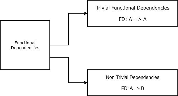
Trivial and Non-Trivial Dependencies
Functional dependencies are classified into trivial and non-trivial dependencies to help reduce unnecessary or unhelpful dependencies. Although trivial dependencies are theoretically correct, they are usually not useful in practical database design.
Formal Definition of Trivial dependencies
A dependency is trivial for X \rightarrow Y if and only if X is subset of Y (Y \subseteq X ).
Examples:
FD_1: A \rightarrow A \space where \space  A \subseteq A\\
FD_2: \{A, C\} \rightarrow C
If X and Y are two disjoint sets than functional dependencies between them is non-trivial. Only non-trivial dependencies are considered meaningful and useful in database design.
Closure of Set of Functional Dependencies (FDs)
The closure of set of functional dependencies (FDs) is the process of finding all the possible FDs that hold for a given relation schema R. It is denoted as F+.
The size of the closure, F+ can be large or small, depending on the number of attributes in the relation and number of interdepenent FDs of relation schema R.
Armstrong’s Axioms
For smaller FDs, it is easier to find the closure F^+ by directly listing all the FDs. However, for a huge relation schema, with trivial FDs , non-trivial FD and redundant FDs, closure of F, F^+ will be huge. To find the closure of set of functional dependencies, F^+, we use a set of inference rules called Armstrong’s Axioms.
The three basic axioms are:
- Reflexivity rule
- Augmentation rule
- Transitivity rule
Reflexivity Rule
If \space Y \subseteq X, then \space X \rightarrow Y
The reflexivity rule means that if Y is a subset of X, then the set of attributes, Y functionally dependent on X. In other words, X functionally determines its own subset Y.
Augmentation Rule
If X \rightarrow Y, then \space ZX \rightarrow ZY for \space any \space set \space of \space attributes \space Z
It means we can safely add a set of attriibutes Z to both sides of the FD. The augmentation rule only allows you to add attributes to both sides of a valid FD – it does not gurantee that the reverse it true.
Transitivity Rule
If X \rightarrow Y \space and \space Y \rightarrow Z , then \space X \rightarrow Z
If a set of attributes X determines Y and Y[/katex[ determines [katex]Z, then X functionally determine Z is called the transitivity rule.
These axioms form the basis of finding the closure of FD and we can also derive additional inference rule from these 3 basic axioms.
Additional Inference Rules (Derived from Armstrong's Axioms)
Addition inference rules are derived from Armstrong's basic axioms and they make it easier to work with functional dependencies. The derived rules are listed below.
- Union rule
- Decomposition rule
- Pseudotransitivity rule
Union Rule
If \space X \rightarrow Y \space X \rightarrow Z , then \space X \rightarrow YZ
It means two dependents ( Y , Z ) with same determinant (X can be combined into one.
Decomposition Rule
If \space X \rightarrow YZ, \space then \space X \rightarrow Y \space \space and \space X \rightarrow Z \space holds
It means any dependency with multiple attributes on right side can be split into smaller groups. The goal here is to split the FD such that we have only single attribute on the right side. There are three reasons for that:
- Its easy to manage the closure of FD with single attribute.
- Some normal forms such as Boyce-Codd normal form need FDs in single attribute form.
- Its very easy to detect redundent and trivial FDs and you can do it manually.
Pseudotransitivity Rule
If \space X \rightarrow Y \space and \space WY \rightarrow Z, \space then \space WX \rightarrow Z \space holds
The usual transitivity is X \rightarrow Y and Y \rightarrow Z, then X \rightarrow is true.
In pseudotransitivity, WX \rightarrow Z holds because WY together determines the attribute set Z (WY \rightarrow Z).
We can generate large FDs from the basic Armstrong's axs and the derived rules from the basic axioms. We need to reduce the closure of FDs, to a smaller size through closure of attributes.
Closure of Attributes (Z^+)
The closure of FDs (F^+)) for a given F, is huge because it runs Armstrong's axioms repeatedly until no more FDs could be generated. We don't need all the FDs in F^+, instead a subset of FDs of F^+ which implies all FDs of F^+ is enough, with needing us to compute the F^+.
Formal Definition of Closure of Attributes
A relation schema R has
- a set of functional dependencies, F of R.
- a set of attributes,Z of R, for which we want to find a closure.
The closure of a set of attributes Z of R, is Z^+. The Z^+ is set of attributes that are functionally determined by Z under F.
How To Find Closure of a Set of Attributes, Z^+ under F
The steps to find closure of a set of attributes, Z^+ is given below.
Step 1: Initialize the Z^+
In the first step, we initialize the by assigning attributes of [katex]Z.
Z^+ = Z
Step 2: Examine all functional dependencies X \rightarrow Y in F iteratively
The step 2 is a loop and it goes through each FD in F.
Step 3: Test if X is a subset of Z^+
As we iterate through each FD in F, we will test whether, right side of the FD is a subset of Z^+.
X \subseteq Z^+
If the condition is true, and X is a subset of Z^+, then add all attributes of Y to Z^+.
Z^+ = Z^+\cup \space Y
Step 5: Repeat Step 3 and Step 4 process for all FDs in F
Continue this to all the FDs in the F, until you cannot add anymore attributes.
Step 6: Display the resultant Z^+
The final Z^+ contains all the attributes functionally determined by Z under F.

Example :
Find the closure of attributes of F = { A \rightarrow B, B \rightarrow C, C \rightarrow D}.
Solution:
Let F = {A \rightarrow B, B \rightarrow C , C \rightarrow D} and Z = {A}
Note that the choice of Z , a set of attribute could be anything. As a database designer, you want to check for a super key or/and find minimum cover (a small set of FDs that implies the same thing as F+). You may like to test different set of Z
Step 1:
Z^+ = Z = {A}Step 2:
We iterate through all FDs and check for condition, Y \subseteq Z^+.
Check A \rightarrow B, since A \subseteq Z^+, add B.
Z^+ = Z^+ \cup B \\
Z^+ = \{A, B\}
Check B \rightarrow C, since B \subseteq Z^+, add C.
Z^+ = Z^+ \cup C \\
Z^+ = \{A , B, C\}
Check C \rightarrow D, since C \subseteq Z^+, add D.
Z^+ = Z^+ \cup D\\
Z^+ = \{A , B, C, D\}
We followed Step 3, 4 and 5 together above to get the final Z^+.
Step 6: Display final results.
Z^+ = \{A, B, C, D\}Equivalence of Functional Dependencies
We know that closure get huge and we don’t need all the FDs, if there is a small set of FDs which implies the same things as F^+, it is called equivalent set of functional dependendencies.
Let there be two sets of functional dependencies, F and H, are said to be , if they implies exactly the same functional dependencies, which means:
F^+ = H^+
How this Helps in Database Design
The equivalence helps in database design in number of ways.
- Simplification – replacing a large set of dependencies with a smaller set increases the efficiency of the database. The smaller set is the “canonical cover” for the larger set. From definition, if a database applies F^+, the equivalent set His also applied. In other words, H is cover for F^+.
- Normaliztion – the use of smaller set is desired in some normal forms such as BCNF or 3NF.
- No Loss of Data – reducing the size of set of FD, , rewriting, deleting FDs, ensure that there is no loss of constraints ,and therefore, no loss of data.
Example:
Let F and H be two sets of functional dependencies where:
F = \{A \rightarrow B, B \rightarrow C \} \\\\
H = \{A \rightarrow B, A \rightarrow C \}
Closure of set of attributes of F
Z^+ = \{A\}\\
Check \space A \rightarrow B, A \subseteq Z^+ \\ Add \space B \\ Z^+ = Z^+ \cup B \\
Check \space B \rightarrow C, B \subseteq Z^+ \\ Add \space C \\ Z^+ = Z^+ \cup C\\
Z^+ = \{A, B, C\}
Closure of set of attributes of H
Z^+ = \{A\}\\
Check \space A \rightarrow B, A \subseteq Z^+ \\ Add \space B \\ Z^+ = Z^+ \cup B \\
Check \space A \rightarrow C, B \subseteq Z^+ \\ Add \space C \\ Z^+ = Z^+ \cup C\\
Z^+ = \{A, B, C\}
The closure of attributes for both F and H are same, they are equivalent set of FDs.
Minimum(Canonical) Cover of a Set of Functional Dependencies (F)
The canonical cover (also known as minimum cover) for a set of functional dependencies F is the simplified equivalent set of functional dependencies without redundancy and implies the same rules as F.
A set of FDs, F_c is canonical cover for another set of FDs, F, if:
F_c \equiv F
and F_c satisfy 3 conditions of minimality.
- Right-hand side of FDs are reduced to single attribute.
- Left-hand side of FDs should not have extroneous attributes.
- No FD can be removed without changing the closure of F, that is, evey FD in F is unique.
We shall explore these conditions in more detail.
1. Right-Hand Side side of FDs are reduced to single attribute.
Given a set of FD, F, each dependency should be in the form, X \rightarrow Y, that is, the right-hand side of FD contains only a single attribute.
If the FD is of the form:
X \rightarrow A_1,A_2, A_3, ..., A_n
Then we should split the FD into following:
F = \{X \rightarrow A_1, X \rightarrow A_2, ..., X \rightarrow A_n\}2. Left-hand side of FDs, should not have extraneous attributes
Each FD in the set of FDs, F has no extraneous attributes on its left-hand side. All attributes on the left-hand side are essential for dependency to hold and cannot be removed them, unless they are redundent.
If the FD X \rightarrow Y has following form with Z = \{A, B\}.
F = \{AB \rightarrow C, B \rightarrow C\}Step 1: Form a new set of attribute Z, where
Z = (X - \{A\}) = \{B\}It means find a new set of attributes without \{A\} without changing anything in the set of FDs, F.
Step 2: Find closure of new Z
Z^+ = \{B, C\}Step 3: Check the condition for extraneous attribute
Y \subseteq Z^+, \space where \space Z = (X - \{A\})We can see that C \in Y and C \in Z^+, therefore, A is extraneous attribute.
If all attributes in Y can be functionally determined from Z (where Z=X−\{A\}), that is, if Y \subseteq Z^+, then attribute A is extraneous in the left-hand side of the FD X \to Y.
3. No redundant Dependencies
There must not be any redundant FDs in the equivalent set of FDs, F_c, since F_c \equiv F, if unique FD is removed than it
will change the closure and equivalence not longer holds.
If a FD f \in F_c:
Step 1: Find a new set of FD,
F_r = (F_c - \{f\})Step 2: Find closure of F_r.
{F_r}^+ = (F_c - \{f\})^+Step 3: Check if f can be derived from (F_c - \{f\})^+
(F_c - \{f\})^+ \nsupseteq fStep 4: If the condition is true and you cannot derive f from (F_c - \{f\}) then fis not redundant. If the condition is false , then FD, f is redundant.
Example
Let F = \{A \to B, B \to C, A \to C\} be set of dependencies and f = A \to C be the FD for redundancy test.
Step 1: Find the new set of dependencies F_r without f.
(F - \{f\} ) = \{A \to B, B \to C\}Step 2: Find closure of the new set of FDs, (F - \{f\}).
(F - \{f\})^+ = \{A \to B, B \to C, A \to C\}Step 3: Check if F is equivalent to the new set of functional dependencies, (F -\{f\}).
F^+ \equiv (F - \{f\})^+Clearly, closure of F is equivalent to closure of new set of functional dependency, (F - \{f\}), which implies that the functional dependency A \to C is redundant. We can discard it safely.
Procedure to Find the Canonical Cover of a Set of Functional Dependencies (F
A canonical cover must satisfy the three conditions mentioned below.
- The RHS of each functional dependencies in F must be a single attribute.X \to A where A is single attribute.
- F must not contain extraneous attributes. If F \to Y is a functional dependency , then X cannot have extraneous attributes.
- No redundant FDs allowed which means F^+ \equiv (F - \{f\})*+.
Example 1
Find the canonical cover for the following set of functional dependencies, F.
F = \{A \to BC , B \to C\}Solution:
For the given F = \{A \to BC, B \to C\}
Step 1: Split the RHS of each functional dependecy into single attributes.
F = \{A \to BC, B \to C\} \space becomes \space \\F = \{A \to B, A \to C, B \to C\} \space after \space splittingStep 2: Check if LHS has extraneous attributes
There is no extraneous attributes in F.
Step 3: Check if there is redundant functional dependencies in F.
Let us remove A \to C and create a new set of functional dependency F_c.
F_c = (F - \{f\}) =\{A \to B, B \to C\}Step 4: Find closure of F_c
{F_c}^+ = \{A \to B, B \to C, A \to C\}The F_c and F are equivalent A \to C is redundant.
The canonical cover for the set of functional dependencies F is:
F_c = \{A \to B, B \to C\}Summary of Functional Dependency in DBMS
A Functional Dependency (FD) defines a relationship between attributes, written as X \to Y, meaning X[/katex uniquely determines [katex]Y.
- FDs are the foundation of normalization and help identify redundant data, anomalies, and keys.
- There are two main types:
- Trivial FD: Y \subseteq
- Non-trivial FD: Y \not\subseteq X
- The closure of a set of FDs (F^+) contains all FDs implied by F.
- The attribute closure (X^+) lists all attributes functionally determined by X.
- Armstrong’s Axioms (Reflexivity, Augmentation, and Transitivity) form the logical basis for all FD derivations.
- A canonical cover (or minimal cover) is a simplified equivalent of a set of FDs that:
- Has only one attribute on the right-hand side.
- Has no extraneous attributes on the left-hand side.
- Has no redundant dependencies.
- FDs are essential for determining candidate keys, normal forms, and lossless decomposition during database design.
- In practice, understanding and simplifying FDs ensures that database schemas are consistent, minimal, and free of anomalies.
Transaction Processing in DBMS: Concepts, Properties and Examples
In real world we do many types of transactions, however, we don’t notice little activities during those transactions. In this article, I will explain the transaction and translation processing with examples. You will learn about benefits and working of transaction processing including different states of transaction processing in DBMS. Let’s begin.
What is a transaction ?
We will begin by this simple question. What is a transaction ? To understand it let’s take a simple example. Suppose you go to an online shop and order a mobile phone , you pay for the phone via online banking or credit card etc and the phone is delivered to your house. The whole sequence of activity to buy a phone till you receive it, is a transaction.
In database management (DBMS), a transaction is logical unit of work that represents some real world event of an organization or an enterprise. These logical unit of work are divided into sequence of operations executed in order and the transaction is completed successfully.
Do you need a transaction processing in DBMS ?
Yes! if it is one or two users working with database, then a transaction processing is not required because we know that database will be in consistent state. However, modern databases are huge and thousands of users are accessing them simultaneously.
We have concurrency control in DBMS to control concurrent access to database The transaction processing does the transaction management executing transaction with large databases and many concurrent users. Due to this type of complexity, DBMS comes with the transaction processing system.
Some common examples are : Railway Reservation System, Banking System , etc.
User and Database views about Transaction processing in DBMS
We know that transaction is logical unit of work, but for database , transaction is database processing with one or more database access operations. I mean that a single operation could be reading bank balance , or reducing the account balance of a user, and/or other operations that affect database. All database operation need access to the database first before doing anything.
Users take some action or a sequence of actions to perform certain operations to get access to the database. These operations are – read, write, modify existing data and delete data.
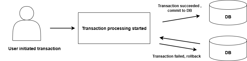
When user or an application begin a transaction, it must be complete which means that the transaction must leave the database in a consistent state. The consistent state is the healthy state of a database. Any other intermediate state is not acceptable.
So, if a transaction begin with a consistent state, after transaction it must leave database in a consistent state. Database transactions are performed using language like SQL. The SQL ( Structured Query Language) is a simple query language for DBMS to translate human queries into machine specific queries and successfully retrieve the results.
We talked about preserving the integrity of the database , to do that any transaction to database must be atomic. It means that when a transaction begin , it must finish successfully or do nothing. A complete transaction should not affect other transactions, even when many other transactions waiting for the same data that current transaction is working on. These are concurrent transactions
The concurrent transactions are also called Serializability. Even though the transactions are concurrent is performed in serial manner in database. This ensures that no other transactions are affected while one transaction is working with the database. Similarly, a transaction can fail, if a transaction failed, it must not affect the database.
What are the benefits of Transaction processing ?
There are numerous benefits of a transaction processing unit in DBMS. But, I am going to list only three primary benefits.
- No inconsistencies – If there is a conflict in transaction by concurrent users , it does not leave database inconsistent. A transaction either finish successfully or failed without making changes.
- System failures – Protection against system failures like power outage, corrupt database, user error is one of the many tasks of DBMS. How is this related to transaction processing ? The recovery mechanism use different techniques to recover data from transactions. These techniques are log-based recover, checkpoints, shadow paging, database replication and point-in-time recovery. Failed transactions are discarded and database keep track of completed transactions.
- Committed Transactions – Once committed, a transaction cannot be reversed or undone because it is written to the database.
Real Life Examples of Transactions
Now that you know basics of transactions and transaction processing . I will give some example that will reinforce your learning. Some real life event is a transaction.
- Withdrawing cash from ATM is a transaction.
- Making an online purchase is a transaction.
- Paying bill for a service is a transaction.
As a human it seems simple to us, but for a computer system or DBMS it is set of logical operations. So each of these transactions are divided in smaller units called operations (Database operations for easier understanding).
Transaction therefore, is a sequence of operations such as READ, WRITE, SELECT or UPDATE the database. You will learn about operations in SQL and how it is done.
Before a transaction begin , the database is in consistent state and after transaction is finished , it leaves the database in a consistent state.
I am giving the impression that transaction always involve a single database, which is not true. A transaction can use one or more database as and when required. Also, we can do transaction processing in a single stream one after another , so there will never be any conflicts or inconsistencies. Since, we have concurrent users and its not practical to transaction processing in a linear way.
Let’s understand transaction processing with real world examples.
Example 1: Withdrawing cash from ATM
In this scenario, we walk into an ATM ( Automated Teller Machine) to withdraw some cash, we use our card, withdraw the cash , collect card and get a slip for balance in our account. This is a familiar scenario for all.
The ATM machine runs a program that is connected to databases that consists of our account information. Since, there are lot of accounts , probable thousands or millions, bank run data centers using a DBMS. So, when you try to withdraw cash from ATM , DBMS perceives it as a set of database operations. A simple transaction of withdrawing cash is set of database operations. Once you receive the cash, the transaction is complete with balance adjusted for your bank account.
Note: walking up to any ATM is not part of the transaction, but its an activity that initiates the transaction of withdrawing or depositing cash, cheque , etc.
ATM Transaction divided into database operations
These are series of steps in order, once last operation is completed, your transaction is completed successfully.
- Inserting ATM card – you insert your debit card for cash withdrawal, the machine won’t accept all cards.
- Selecting language to communicate – to facilitate easy communication during transaction, you get to choose the language.
- Entering Pin for authentication – this verifies that you are the true account holder authorized to withdraw cash. In other words, do database transaction.
- Choose the Transaction type – ATM allows multiple type of services, not just withdrawal.
- Choosing Account type – your account could be minor account, saving , or current account. Select the right option , so that transaction may continue. This is an added layer of security.
- Choose Amount – Assuming that you want to withdraw, input the correct amount and this will be subtracted from account balance in the database.
- Collect Cash – collecting cash is not database operation, but it indicates that your account balance is adjusted for the withdrawal amount. The transaction is complete.
- Collect receipt – this is ATM getting information from database about your account status and balance.
- Take your card back – transaction is successfully completed.
Once all the steps are completed , your transaction is complete. However, there are constraints for transaction. You must correctly authenticate with pin, withdrawal limits, etc.
Example 2: Purchasing a movie ticket online
This is a common scenario, where you go online to book ticket for a movie. You visit the booking site such as Bookmyshow in India, or SM Cinema in Philippines, or Cinepolis in USA. You visit the website , choose your location, select your movie that you want to watch, select movie hall, type of seats, number of seats, and pay online and you will get the booking confirmation successfully.
Similar to our ATM system, the movie operators or websites also maintain a database that is frequently updated when people buy movie ticket. There are certain constraints. For example, you cannot buy tickets after a show is full and/or after 15 to 60 min of screening, booking stops.
A database transaction for buying movie ticket is limited to selecting location, movie hall, seats and paying for those seats and final confirmation in the form of an online ticket sent to your mail.
Purchasing movie tickets database operations
The process of booking tickets starts with you logging into the booking app or website. Though it is not part of actual transaction, but it initiates the transaction, just like you visiting ATM.
- Selecting location – In this step, you visit the website and then select your preferred location to watch a movie. You simply choose from available locations from a list.
- Select available movies – Select a movie, that you like to watch.
- Select movie hall – The selected movie might be showing in different halls at different timings. You can select the your preferred hall. Though sometimes, the choice depends on timings. You may select a hall because of timings of the show.
- Select number and type of seats – This is the most crucial step, you must select the number of seats, type of seats and any other features available.
- Make payment for seats – Now you make an online payment using any one of the payment gateways available or use a card complete the transaction.
- Seat confirmation – This is an important step as it marks your completed transaction. The database for movies and shows will be updated for those seats that you have booked and you will receive an invoice or ticket in digital form for identification.
The booking movie tickets online is similar to ATM cash withdrawal , only database structure and information are different. In case of failure in completing the booking process, the entire process is roll-backed. You must start the process again. Any amount reduced from your bank account will be reversed automatically.
Example 3: Paying bills online
Our third example is a database transaction where you don’t buy any product, but pay bills for services already received. That is also a kind of transaction. For example, you want to pay for your monthly mobile phone bill. First you need to know, how much money you have to pay ? and any additional charges.
You initiate the transaction by login into the service website, then you select one of the payment methods, pay the bill amount and if the transaction is successful, you will get an acknowledgement in the form of digital receipt. There are so many services you can pay in similar manner.
For database login into the web system is not part of transaction itself, however, it is part of database security. Before executing the your transaction, you must authenticate your self with necessary permission.
Paying bills online as database operations in DBMS
As I mentioned earlier, all transactions are divided into logical operations on one or more database. The process of paying bills online is also divided into logical operations.
- Login into the website – Suppose you are paying bill for your telephone or mobile services. The first thing you do is login into your account on the website.
- View bill to be paid – You get the information about bill that was generated. Sometimes bills could be downloaded as a document like pdf file or word document. The main goal is to know the amount you need to pay including any taxes.
- Select any payment method – Getting bill information is part of database operation , but not selecting the payment method. But, it part of transaction – a task.
- Pay the bill – After you choose one of the online method, pay the bill. If transaction is successful, you will get the confirmation.
- Reference number or receipt – Once the bill is paid , you will receive a transaction reference in your email or a receipt online. This indicates that your transaction was successful. The database is updated with new status of your mobile service. The back account is subtracted by amount mentioned in the bill.
Note: similar to purchasing product or ATM , if transaction is failed, rollback will happen. Only when it is successful, the database is updated permanently.
States of Transaction Processing in DBMS
If the transaction is completed, then it is committed. Any failure of database cannot erase the committed information. It means that committed is a state of transaction processing. There are four main states of transaction processing and each successful or failed transaction goes through these states.
- Active state
- Partially committed state
- Committed state
- Failed state
- Aborted state
- Terminated state
The transaction moves from one state to another until it is terminated after success or failure.

Figure 2: States of a Transaction
Exam focus:
Explain Transaction states with diagram.(3 – 5 marks).
Active State
The active state is where all operation such as read and write happens. Yet, it is not committed to database, and kept in a temporary buffer.
Partially Committed State
In partially committed state, the transaction has completed all the final operation and ready to commit. It is not committed, but getting ready to commit. At this point, any kind of failure in transaction will result in rollback.
Committed State
After writing all changes to the database, a transaction enters the committed state, the changes are written permanently to the database store and cannot be undone. A rollback is not possible in case of failure, but its not required at all because database is updated with the change and its never lost.
Failed State
A transaction enters the failed state when a power failure happens, or a logical corruption in database occurs, or one or more database constraints is violated. The failed state indicate that a transaction cannot be completed successfully.
Abort State
If the transaction has entered failed state , then it must enter the abort state next and rollback the changes. Suppose the failure or error is fixed, that does not mean that transaction will leave failed state and start with an active state automatically. If transaction has failed state, it must rollback first and a new transaction must be initiated.
Terminated State
Whether transaction has committed successfully or aborted due to failure, it is marked as completed and when it enters terminated state , transaction is removed from the system.
“Want a quick summary of Transaction States in DBMS with examples? Check out our Mini-Post version here.”
Next, we will see important properties of transaction processing.
Explain the difference between Failed state and Rollback state (1–3 marks).
Properties of Transaction Processing
The four different properties of database transactions are called ACID properties They stands for
- Atomicity
- Consistency
- Isolation
- Durability
The acid properties ensure that the database transaction processing is reliable and secure.
Atomicity
Think of transaction as one task and all operations must finish within one transaction or nothing should happen and transaction is aborted. In other words, a transaction is multiple read and write operations grouped together. It works on the principle of “All or Nothing”.
Consistency
A transaction must leave database in a stable consistent state with all the new updates, or if the transaction failed for reason, it must rollback all the changes and leave database consistent as it was before the transaction started.
Isolation
During the execution of a transaction, no other transaction is allowed to see the updates or change it, until the current transaction is completed or aborted. The read and write access for data is suspended for any transactions other than the current transaction till it commit successfully and completed.
This kind of system is used in multi-user databases and isolation is achieved through concurrency control.
Durability
Durability means something that stays for a long time. Once the changes are made to the database, it is permanent and cannot be erased by a failed transaction or power failure or a system failure. The database may become inconsistent, however, database management has several recovery mechanisms to bring database back to a consistent state.
Explain ACID properties with example.(3 – 5 marks).
Want to learn about ACID properties in detail. Here is our mini-post version: ACID Properties in DBMS.
SQL and Transaction Processing
As mentioned earlier, SQL is the language of database management and its a structured query language. Usually, you can execute simple insert, select, update or delete individually and get results. In the case of transaction processing, you need distinct commands that the regular read or write.
In SQL , the transaction processing is achieved through three commands;
- BEGIN or BEGIN TRANSACTION
- COMMIT
- ROLLBACK
The BEGIN or BEGIN TRANSACTION marks the start of a new transaction and whatever commands follow it part of that specific transaction. The COMMIT is executed when all the changes are completed in the buffer. The ROLLBACK command is executed when a transaction fails or enter the failed state mentioned earlier.
There are other related commands such as SAVEPOINT. It is a checkpoint to which you can ROLLBACK in case of failure. The checkpoint in part of transaction log about which you will learn in next section.
Transaction Logs
Earlier I mentioned that a transaction is executed in buffer cache, before it is written to the disk and marked committed. The transaction log works with buffer and it is a record of all transaction and changes made to the database. It is not yet written to the database.
What is the use of such a transaction log ? It helps in database recovery using checkpoint. The Log information is used by DBMS for recovery triggered by a ROLLBACK command due to system crash, power failure or abnormal termination of a program.
What are the contents of Transaction log?
In database systems like PostgreSQL, MySql, Oracle and SQL Server , the structure of transaction log is almost the same, which includes following;
- Transaction ID – this is a unique identifier for the transaction and it also mark the beginning or transaction.
- Operation Records – this contains log records with information about type of operations(INSERT, DELETE, etc), table or row that was changed, undo/redo information if a rollback or commit is required.
- Undo/Redo Information – Undo log is information to rollback changes, and Redo log is enough information to reapply committed changes but not written to the disk.
- Long Sequence Number (LSN) – A sequence number that for each records in a transaction log for the purpose of ordering changes in the database. With each operation in the transaction , LSN increment monotonously.
- Commit or Rollback Records – a special record that get updated when transaction commits or rollbacks.
- Checkpoint Records – a specific checkpoint for database recovery so that recovery don’t need to go through entire log.
Test your self : Transaction Processing in DBMS: Concepts, MCQs and Questions
Summary
Let’s summarize what you learned about transaction processing. A transaction is representation of a real life event in the database with one or more database operations. A transaction must finish all operation or do nothing and terminate. Once committed the information in database is permanently stored.
Every transaction goes through different states mentioned in the table below.
| Transaction State | Meaning |
| Active state | Transaction has started |
| Pre-committed state | Transaction has finished all operations and ready to commit |
| Committed state | Transaction has written to the database and committed |
| Failed state | Transaction enter failed state due to failure in processing |
| Abort state | Transaction is rolling back the changes with the help of checkpoint |
| Terminated state | Transaction is removed from the system |
In a multi-user system, every transaction must adhere to ACID properties. The ACID properties and its meaning given below.
| Property | Meaning |
| Atomicity | Each transaction and its operations must be unique |
| Consistency | If transaction commits or rollback in failure , must leave database stable and consistent |
| Isolation | Once data accessed by a transaction , no other transaction must see or change the data until current transaction is finished |
| Durability | Transaction once committed, the information is stored permanently and cannot be undone |
Transaction uses SQL commands and transaction logs to complete its database operation.
Preparing for DBMS university or GATE exams? Revise Transaction Processing in DBMS using a structured, exam-focused PDF that includes:
- Concept overviews
- MCQs
- Short exam questions with solutions
Introduction to DBMS
Think about small data like phone numbers of friends, grocery items list, etc. It is easy to store these information on a piece of paper and retrieve when you need them. An individual can manage it well. Now imagine a large organization that store huge number of data year after year. They need to setup an information system that store , update it regularly, secure, reliable and people should be able to retrieve it quickly in an efficient manner. The core of such an information system is the database management system. In short, DBMS.
This database system has a single goal and it is to provide a consistent environment to store, update and efficient retrieval of data in an organized manner. Other operations of database system is to secure the data servers, and take various security measures, give concurrency control to database, which means manage access to database by multiple users at the same time, database recovery in case of crash, or failure of database servers. Its not necessary that data is always stored on a servers, because an information system can contain various types of storage hardware.
Now that you understand core function of a database management system or DBMS. Let’s talk about most important component of this system – the database.
“A database is structured collection of related data”.
I have to elaborate the definition. Here structured collection means that the data is organized in such a manner that it make storage easy, and retrieval efficient and faster.
The word related data is referring to the type of data stored which may be images, records , or database of audio/video files. The data is related because of its shared attributes or common properties that help in categorizing data in the form of a database.
Tasks Performed by a Database
You know what get stored in a database from its definition. To maintain a consistent database with updated information, it has to perform certain tasks. These are
- Add files to database that store information permanently.
- Add data to files in the form of records, relations, and various logical structures.
- Help retrieve data for users and applications including database administrators.
- Update new data.
- Delete data from files.
- Remove database files if necessary.
The tasks are called basic database operations of DBMS. Data record creation, reading data, updating data and deleting data are core functions to maintain databases.
There are other features about database management systems which I will discuss in next sections.
Features of DBMS
In modern database systems , you will find three common features listed below.
- Data Independence
- External Schema or Views
- Query Mechanism
Each of these features enable database operations , manage consistent database , efficient data retrieval and security to database systems. I will briefly discuss each of these features just enough for you to understand and later on I will elaborate on these topics in a different article.
Data Independence
The idea of data independence is very simple idea that we should able to modify database schemas or database levels without affecting the higher level schemas. A schema is structure and organization of the database at three levels.
- Physical Schemas
- Conceptual Schemas
- External Schemas
The physical schemas are related to how database stores information physically, and database indexes for quick searches. The level above physical schema is the conceptual schemas or logical schema. The external schemas are above logical schemas and it is the highest level of three level schema structure.
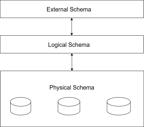
The ability to change the structure of physical schema without affecting higher schemas like logical schema or external schema is called physical data independence. Physical data independence is also called the internal data independence.
DBMS query is a user request to manipulate databases and these user requests are translated / executed using a Structured Query Language (SQL). Each database query must go through three process
Similarly, you can modify or change structure of conceptual schema (logical schema) without affecting the higher external schema which is knowns as logical data independence. If the logical data independence is achieved , it is also external data independence because it does not require you to change the external schemas or user views.
External Schemas or Data Views
The external schema or views are highest level of database abstraction. It simply means that you can create more views or tables from the same database different from logical schema and/or physical schema.
Users of external schema don’t have or want to do anything with how data is stored in the database. A particular external view only shows them, what they need to know. Not only that , but DBMS also allows you to create multiple views from same database.
For example, A bank account holder will see only his account details such as bank balance and transaction history etc. On the other hand, a bank manager will see overall status of accounts and customer personal information. One aspect of view is access privileges’ which decide how much and which views a user get to access. You doing Google search and search results on the page is also a external view , totally different from how Google store websites information.

External schemas can stay the same, yet when application using them or user change the data , that is reflected in the logical schema. This is external data independence.
Another advantage of external schema and its independence from conceptual schema and physical schema is data security. With limited access to information, database administrators can protect sensitive information from threats or unauthorized access.
Query Mechanism (SQL)
- Parsing or Translation
- Execution
- Query Optimization
The Query parsing is a process to check syntax error in SQL command called the syntax checking, then the parser checks for semantic errors meaning does the database and table exists, compatibility of query, etc. If the query is passed all checks, it translate the query to relational algebra or a query tree, both of which are internal representation of query for optimization.
The query optimization is to prepare the query for efficient execution by reducing time and resources to execute the queries. Finally, the query is executed and precise results are fetched.
To understand the advantages of DMBS system let us compare it with older version of database system. There were no systems to store data and earlier database applications were build using the computer file system. In other words, data were stored in files and accessed directly.
File System vs. DBMS
Like file system, DBMS also stores data in files, but it provides a system to manage it well using three tier-schemas. Then there is additional security and concurrency control.
The traditional file system has few problems with storing data which are:
- Duplicates data – sometime files or duplicated entries cause problems with application or users. Sometime users create multiple files with same name or enter duplicate entries that can cause confusion or give erroneous results. In DBMS, each record is given a unique id to prevent duplicates.
- Change in one file is not reflected in other files – Since multiple users access the files and change it continuously, sometimes they are not synced together and you may find difference in data because it is not updated on other files. With DBMS system, change in relations or views, it either Updated or terminated completely.
- Multiple file formats – With traditional file system, files are often stored in multiple formats and that will limit the data independence and increase costs of maintaining such a system.
- Database Integrity problems: Database integrity refers to consistency, accuracy and reliability of database and it is enforced using database constraints which are nothing but rules for databases. With file system, adding constraints or modifying them such as file size, user permissions, etc. With DBMS system, there are fewer constraints management and they are easy to implement.
- Atomicity : DBMS transactions to database are atomic, means they either succeed or fail , so the database is always consistent and safe. With file system, failure of database can leave the database in inconsistent state.
- Concurrent Access Problems: The traditional file system is not good at handling multiple users concurrently accessing the database, two user can access the same data and leave the wrong entry.
- Security: It is very difficult to ensure file security and security constraints in traditional file system.
DBMS Solution to all the above mentioned problems:
- Logical storage reduce space, time to access data and complexity. The logical storage also prevents duplicated and updating time.
- It has indexes to do faster searches and special data structures for faster retrieval of data.
- Simple as well as complex queries through SQL is possible.
- Database Integrity constraints are handled efficiently.
- Backup and Recovery system.
- Database security by restricting users based on roles and permissions. Only authorized users can do certain high level tasks.
- Multiple User Interfaces for different types of users. For example, menu-based, form based interfaces and GUI( graphical user interfaces). There are separate interface for database administrators.
Summary
The DBMS system stores data in organized manner and performs database operations on them such as Add, Update, Delete or Modify.
Database has three-level architectures that provides full data independence. One level need know activities of higher level schemas. Apart from that DBMS is provides database security, concurrency access and backup and recovery system.
Database queries are handled through an easy and simple query language called SQL ( Structured Query Language).
Finally, I mentioned the difference between traditional file system database and DBMS. The solution provided by DBMS is robust and efficient.
Database Management (DBMS) Notes – Concepts, Examples, MCQs & Exam-Ready Revision
Database Management System (DBMS) is a core subject in Computer Science and IT courses as well as competitive exams like GATE, UGC NET and university exams.
On this page, you will find structured resources to learn DBMS concepts, along with clear explanations, examples and exam-ready revision notes.
What will you learn
On this page you will find:
- Core DBMS concepts explained clearly and systematically
- Exam-oriented explanations supported with relevant examples
- MCQ-based practice posts to test your understanding
- Detailed articles along with exam-ready revision PDFs
This Page is for:
- Computer science and IT students
- GATE and other competitive exam aspirants
- University exam preparation
- Self learners
Topic Sections
Find DBMS topics here.
(1) DBMS Fundamentals
(2) ER Model & Database Design
(3) Relational Model
(4) Relational Algebra & Relational Calculus
(5) SQL
(6) Functional Dependencies
(7) Normalization
(8) Transactions
(9) Concurrency Control
(10) Recovery System
(11) Indexing
(12) File Organization
(13) Query Processing
🎁 Get the SQL Starter Kit (Free for Students)
Build your SQL foundation with these three essential PDFs:
- SQL Basics Explained
- MySQL Installation Guide
- SQL Practice Questions (20 problems)
This starter kit is free, but requires a quick signup so we can send the PDFs directly to your inbox.
👉 Sign up and receive the download link instantly