Operating Systems Archives - Page 2 of 4

File Concepts

To a user, the file is the smallest unit of storage on a computer system. The user performs file operations such as open, close, read, write and modify. They can create or delete files from the system. In this article, you will learn the basics of file and file system.

File Concept

Computer store information in storage media such as disk, tape drives, and optical disks. The operating system provides a logical view of the information stored in the disk. This logical storage unit is a file.

The information stored in files are non-volatile, means they are not lost during power failures. A file is named collection of related information that is stored on physical storage.

Data cannot be written to a computer unless it is written to a file. A file, in general, is a sequence of bits, bytes, lines, or records defined by its owner or creator. The file has a structure defined by its owner or creator and depends on the file type.

Text file – It has a sequence of characters.
Image file – It has visual information such as photographs, vectors art and so on.
Source file – It has subroutines and function that are compiled later.
Object file – It has a sequence of bytes, organized into bytes and used by the linker.
Executable file – The binary code that the loader brings to memory for execution is stored in an exe file.

File Attributes

A file has a single e editable name given by its creator. The name never changes unless a user has necessary permission to change the file name. The names are given because it is humanly understandable.

The properties of a file can be different on many systems, however, some of them are common:

Name – unique name for a human to recognize the file.
Identifier – A unique number tag that identifies the file in the file system, and non-human readable.
Type – Information about the file to get support from the system.
Size – The current size of the file in bytes, kilobytes, or words.
Access Control – Defines who could read, write, execute, change, or delete the file in the system.
Time, Date, and User identification – This information kept for date created, last modified, or accessed and so on.

The information about the file is kept in a directory structure which also resides on the secondary storage.

File Operations

The operating system performs the following file operations using various system calls:

Create
Read
Write
Delete
Reposition
Truncate files

Create Files – User must have necessary disk space on the file system to create a file. A directory entry is required where the file is created.

Read Files – The system call requires file name and next block in memory to be read. The system needs a read pointer to read the file from a specific location in the file and this pointer is updated for the next read from the file.

Write Files – The system call uses same file pointers of the process to write to a file. This saves space and reduces complexity.

Repositioning within a file – The current-file-position pointer is repositioned to a given value. It does not involve an I/O, and known as file seek operation.

Deleting a file – We look into the directory for the file name, if a file is found, release the space occupied by the file and remove directory entries for the deleted file.

Truncating a file – Sometimes the user does not want to delete a file, but remove some information from it. This will change file length attribute, however, other attributes remain unchanged.

There are other file operations such asappending a file,renaming a file, create a duplicate copy of the file.

Open-File Table

The file operations require searching a directory every time. To avoid frequent searches, the OS allows a system call – open() and keeps an.open file table When the file operation is requested, the system refers to the file via an index value. The file is not used actively, the process closes the file and the OS remove its entry from the open file table.

The open() system call can take mode information such as read-only, write, append, create, and so on. The mode is checked against the file permission and it allowed file is open for the process.

The open call returns a pointer to the entry in the open-file table and the pointer, not the file is used for all I/O operations.

Several different files may open the same file, therefore, the system maintains two file-tables – per-process table and system-wide table. The per-process table contains information about files opened by the file.
For example, current file-pointer for each file, access rights, and accounting information for the files.

Each entry in the process file-table points to a system-wide table, which contains process independent information such as the location of the file on the disk, access dates, and file size. When a process opens a file, an entry is added to the processor open file table of the process and points to the entry in the system-wide table.

The open file table keeps an open count indicating the number of processes that have opened the file. The close operation decreases the count and when it reaches 0 the file entry is removed from the open-file table.

The following information is associated with an open file:

File pointer – It helps in read() and write() operation. It is unique to each process.
File Open count – When multiple processes open the same file, therefore, file open-count keep track of open files and closed files and when the count reaches 0 and process can remove the entry from the open-table.
Disk location of the file – To modify data the path to the file is kept in memory. The system does not have to read it for each operation.
Access rights – The process opens the file in access mode and information regarding the access rights is in the per-process table, based on which OS can reject or accept the I/O request.

Apart from the above, some OS provides ways to lock files. This is true in the case of shared files where only one process can write to the file while other processes read the information on the file.

References

Abraham Silberschatz, Peter B. Galvin, Greg Gagne (July 29, 2008) Operating System Concepts, 8 edition edn., Wiley.

post

Paging

Paging allows the physical address space of a process to be non-contiguous. It avoids the external fragmentation and there is no need for compaction.

Fragmentation problem affects the backing store (disk) of the main memory where processes are swapped in or out. The compaction is not possible due to the slow access speed of the backing store. The paging method solves this problem by storing chunks of memory in the backing store.

The paging is supported by paging hardware, but recently paging is done both by operating system and hardware, especially on 64-bit microprocessors.

Basic implementation of Paging

The physical memory is broken into fixed-sized blocks called frames and logical memory is broken into blocks of the same size called. Pages.

When a process is executed, its pages are loaded into available memory frames from file or backing store. The backing store is also divided into blocks of the same size as frames. Every process contains its own page table. Not all pages are sent to physical memory, only a few pages called working set are loaded into the physical memory or
frames.

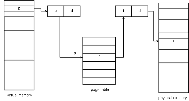
Figure 1 – Virtual Address and Physical Address

Every address generated by CPU is divided into page number (p) and page offset (d). The page number is used as an index into a page table The page table contains the base address of each page in physical memory which is combined with the page offset to define the physical memory address that is sent to the memory unit.

Figure 2 – Page Table

The size of the page is a power of 2, varying between 512 bytes to 16 MB per page, depending on computer architecture.

Virtual Address Translation

The page contains logical address spaces; hence, the logical address space must be translated into a page number and page offset.

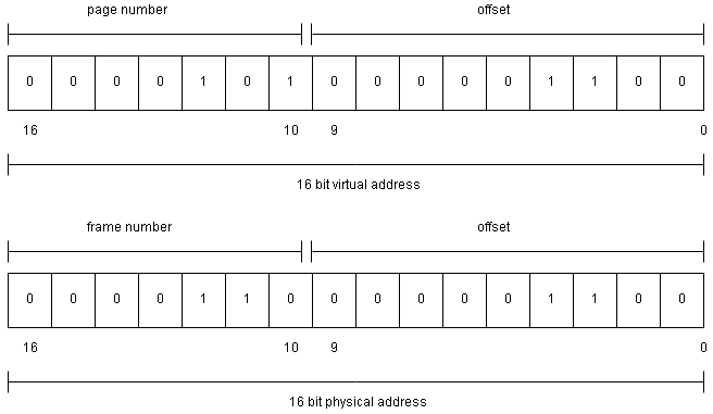
Suppose the virtual address is 16-bit address and page size is 512 bytes. Then:

Virtual address = (page_number * maximum_offset_value ) + offset_value

maximum_offset_value = 512 bytes
offset value = log2 (512) = 9 bits
page_number = 16 - 9 = 7 bits

The virtual address higher order 7 bit is used for the page number and lower order 9 bit is reserved for offset_value.

Example:

The 16 bit virtual address is split into page number and offset value.

0000011 000000110 = (page_number, offset) = (3, 6)

Therefore, memory address location = 3 * 512 + 6 = 1536 + 6 = 1542

For 16-bit physical memory address, the higher order 7 bits represents frame number (f) and the offset value (d) is same for the physical address as the virtual address.

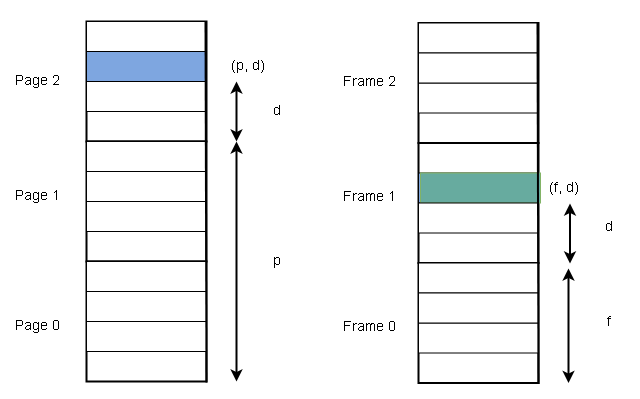
Figure 3 – Virtual Address Space and Physical Address Space with Paging

Example:

00000100 00010000 = (frame_number, offset_value) = (4, 16)
physical memory location = [(frame_number * maximum_offset_value) + offset_value]

Therefore, frame memory address location = 4 * 512 + 16 = 2048 + 16 = 2064

The physical address must equal to or greater than the virtual memory. If there are n pages then at least n frames are required. Each page requires only one frame. The mapping is hidden from the users. The address mapping is done using address-translation hardware.

Page Table

We already know that a page table is indexed on page numbers. In its simplest form, a page table contains the frame numbers with the offset value gives the physical address and its location in page frame.

You will learn more about the page table in the next article.

Internal Fragmentation vs. Page size

There is no external fragmentation because any free frame is allocated to a process in execution. But we there may be internal fragmentation.

For example, if page size = 2048 bytes
process size = 72766 bytes need 72766/2048 = 35 pages + 1086 bytes

The process will be allocated 36 frames for 35 pages, resulting in an excess of 2048 – 1086 = 0962 bytes wasted space. Smaller page size means less internal fragmentation, however, page table entries increase leading to more page table overheads.

The page size in recent years have increases between 4 KB to 8 KB and some system support larger pages. This is due to the larger main memory sizes. The larger page table entries have two advantages – less disk I/O and less page table entry overheads.

Example:
Solaris uses 4 KB and 8 KB pages.

Frame Table

When the process is executed, the pages are allocated frames. The operating system keeps track of physical memory by listing free frames, frames not available, number of frames and so on. It does that with the help of a data structure called the frame table.

Figure 4 – Frame Table

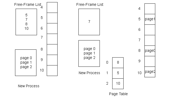
The frame table has one entry for each page frame. The entry indicates whether the frame is free or allocated, if allocated, then the process and the page number.

References

The University of Texas () Virtual Memory, Available at: http://www.cs.utexas.edu/users/witchel/372/lectures/15.VirtualMemory.pdf (Accessed: 5/23/2019).
Abraham Silberschatz, Peter B. Galvin, Greg Gagne (July 29, 2008) Operating System Concepts, 8 edition edn., : Wiley.

post

Contiguous Memory Allocation

The contiguous memory allocation uses memory partitions to allocate memory. These partitions could be fixed or variable size partitions allocated according to first fit, best fit, or wort fit method. The memory fragmentation is a common problem that affects these partition memory allocation system.

Contiguous Memory

Contiguous memory allocation is a method of allocating memory to OS and user processes. The memory is divided
into two partitions

1. For resident OS.
2. For user processes.

The OS can be placed in lower memory or higher memory, it is usually in the lower memory because the interrupt vector
is placed in lower memory. We want to allocate memory to several processes at the same time, therefore, each
process is allocated a single contiguous section of memory.

Contiguous Memory Allocation Methods

The simplest method of memory allocation is to divide memory into fixed-sized partition. Each partition may or may
not contain exactly one process. When a partition is free, a process is selected from the input queue and loaded into
the fixed partition. The memory is available again when the process terminates.

Example:

IBM OS/360 called MFT used this method.

There is another way of allocating memory is using variable partitions. The OS keeps a table of occupied memory
and free memory. Initially, when no process is running in userspace, it is one large block of free memory called a
hole.

In this scheme, the process scheduler selects a process from the input queue and consider the following:

The memory requirements of the process.
Compute the available memory for user processes.
Allocate memory and load the process for execution.
If there is not enough memory to accommodate the process, OS waits for memory to be available, or swap the
process with a smaller one from the queue with smaller memory requirements.
There are a lot of smaller adjacent holes of various sizes, OS can combine those to form a bigger hole to allocate memory to process.
The OS can split a larger hole to create smaller holes for processes.

Strategies To Allocate Free Memory Holes

The operating system search for a free hole for the process of size n from available free memory. The first-fit, best-
fit and the worst-fit strategies are used to select a free hole.

First Fit Method:

Allocate the first hole that is big enough for the process. Either start looking from the beginning of a memory or start where previous first-fit allocation ended. Stop the search as soon as a match is found.

Best Fit Method:

Find the smallest hole that is big enough to fit the process.

Worst Fit Method:

Find the largest hole for the input process.

Memory Fragmentation

The memory fragmentation is a problem of little pieces of memory that cannot be used and wasted during dynamic memory allocation.

Internal Fragmentation:

The internal fragmentation is caused due to unused leftover space within a partition. For example, if a process requests for a hole size of 15340 bytes and the hole size of 15344 bytes is available. The leftover would be 4 bytes which are completely wasted.
A solution to this problem is to split physical memory into blocks of equal size and allocate block sized memory to process slightly larger than the requested memory. This will reduce the unused memory internal to the block partition.

External Fragmentation:

The external fragmentation happens when processes are allocated memory using best fit or first fit methods. The memory becomes non-contiguous and broken into smaller pieces. The problem of external fragmentation could be severe such that there is a lot of fragmented pieces of memory between two processes.
A solution to external fragmentation is compaction which brings all free memory together making one large block of a free hole. This solution is possible at run-time only. If possible then we could relocate all running process to one direction and free holes in other direction.

The other solution to external fragmentation is to allow virtual memory to be non-contiguous and allocate physical memory when available. This scheme is called paging.

References

Abraham Silberschatz, Peter B. Galvin, Greg Gagne (July 29, 2008) Operating System Concepts, 8 edn., Wiley.
Ramez Elmasri, A Carrick, David Levine (February 11, 2009) Operating Systems: A Spiral Approach, 1st edn., McGraw-Hill Education.
Tanenbaum, Andrew S. (March 3, 2001) Modern Operating Systems, 2nd edn., Prentice Hall.

post

Dynamic Loading And Linking

To run a process, the entire process and its data must be in physical memory. Thus, the size of a process is limited to the size of physical memory. The dynamic loading and linking are run-time operations.

Dynamic Loading

The dynamic binding is a method to obtain better memory-space utilization. A routine is not loaded until it is called, until then all routine remains in the disk as relocatable code format.

A routing can call another routine, but it checks if another routine is loaded or not. If not, then relocatable linking loader is called to load the routine into memory and update program’s address tables to reflect this change. The control is passed to the newly loaded routine.

The total program may be large but only a small portion is loaded. The unused routine is never loaded into memory.

It is the programmer’s responsibility to implement dynamic loading, the OS can provide library routines to implement the dynamic loading.

Dynamic Linking

In static linking, the system libraries are treated like any other object modules and combined by the loader into the executing program.

The dynamic linking, similar to dynamic loading is delayed until run-time. This feature is used with system libraries such as language subroutine libraries. Without this facility, each program must include a copy of its language library in the executable image which wastes memory space.

There are several benefits of dynamic linking:
– library routines not part of program code. A program is much smaller without the routines and loads faster into the memory.
– One copy of library routing is referred by many programs, therefore, saving disk space and memory space.
– Fixing bugs is easy because you are only required to fix a single routine, rather than individual copies of it.

The library can be updated with a newer version. Since the program must use the correct version of the library, the version information is included with the program and the library. Also, several version of the library is loaded into the memory, so that programs could use the correct copy of the library.

If the library has minor changes it retains the same version number. The version is incremented if the library has major changes, and affects the only program that is compiled using a newer version of the library. Old programs use an older version of libraries. This system is known as shared libraries.

Libraries require help from the operating system. If the processes in memory are protected from one another, OS checks if the required routine is already linked to another process, or allow multiple processes to access same memory addresses.

References

Abraham Silberschatz, Peter B. Galvin, Greg Gagne (July 29, 2008) Operating System Concepts, 8 edn., : Wiley.
Ramez Elmasri, A Carrick, David Levine (February 11, 2009) Operating Systems: A Spiral Approach, 1st edn., : McGraw-Hill Education.
Tanenbaum, Andrew S. (March 3, 2001) Modern Operating Systems, 2nd edn., : Prentice Hall.

post

Logical Memory Address vs. Physical Memory Address

The memory binding could be static or dynamic. In dynamic binding system, user-generated virtual addresses are mapped to physical addresses. This leads to better memory utilization.

The address generated by CPU is called a logical address, and the address seen by the memory unit is called a physical address. The physical address is loaded into the memory-address register of the memory.

Logical vs. Physical Address

The compile-time and load-time address binding generate identical logical and physical address due to static binding techniques.

The logical address and physical address are part of the runtime address binding technique. They are different from each other. The logical address is also known as a virtual address. The virtual addresses are pages of fixed or variable size and the physical address are called frames that are part of memory hardware (RAM).

Memory Relocation and Address Spaces

Set of all logical addresses by a program is called its logical address space. Set of all physical addresses corresponding to physical address is called physical address space. The run-time mapping is done by hardware called the memory-management unit (MMU).

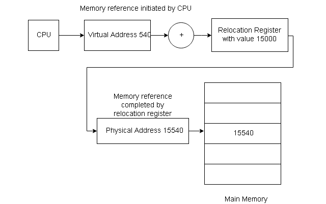
Figure 1 – Memory Relocation Register

A simple MMU scheme is to change base register to relocation register. The value in the relocation register is added to every address generated by a user process (virtual address).

For example, if base = 15000, then access to location 540 is mapped to 15540 (physical address). MS-DOS with an intel 8086 used 4 such relocation registers to run processes.

The program uses the logical address to do all memory operations using virtual address e.g 540 without knowing the physical address e.g 15540.

Only when used as a memory address, it is relocated using relocation register and reference is completed by fetching physical memory address. The final location of the referenced memory address is not known until a reference is made.

So now, when user programs run, each program thinks that it has 0 to 2^N memory, but it must be mapped to (R+0) to (R + 2^N) with a base register value of R.

This logical address space binding to physical address space is the main concept of memory management.

References

Abraham Silberschatz, Peter B. Galvin, Greg Gagne (July 29, 2008) Operating System Concepts, 8 edn., : Wiley.
Ramez Elmasri, A Carrick, David Levine (February 11, 2009) Operating Systems: A Spiral Approach, 1st edn., : McGraw-Hill Education.
Tanenbaum, Andrew S. (March 3, 2001) Modern Operating Systems, 2nd edn., : Prentice Hall.

post

What is a Deadlock?

In a multiprocessing environment, several processes compete for limited resources. A running process goes to waiting state when a resource is not available. The process could not change its state because some other process holds the resources. This is called a deadlock.

Normal Conditions

The operating system does not provide with deadlock prevention mechanism, the programmers must write deadlock-free programs.

Under normal circumstances a process utilizes resources in the following way:

The process request for the resource, and must wait if the resource is not granted immediately.
The process once allocated the resource, can operate on it.
The process must release the resources once finished execution.

The list of system calls used to manage resources via system calls are:

request ()
release ()
open ()
close ()
allocate ()
free ()
wait ()
signal ()

Necessary Conditions for Deadlock

A deadlock happens if four of the following condition hold simultaneously in a system:

Mutual exclusion
Hold and Wait
No Preemption
Circular wait

Mutual Exclusion

Only one process can use the resource at a time. The process must not share the resource with another process. If the resource is requested by another process then it has to wait until the resource is released.

Hold and Wait

A process must be holding at least one resource and waiting for additional resources that are held by other processes.

No Preemption

The resources held by the process cannot be preempted and it can only be released by that process after completing its tasks.

Circular Wait

A set $\{ P_0, P_1, \cdots ,P_n \}$ of waiting processes exist such that $P_0$ is waiting for resource held by $P_1$ , $P_1$ is waiting for $P_2$ , $P_{n-1}$ is waiting for resource held by $P_n$ , and $P_n$ waiting for resource held by $P_0$ . This situation is called circular wait, and also known as hold-and-wait.

References

Abraham Silberschatz, Peter B. Galvin, Greg Gagne (July 29, 2008) Operating System Concepts, 8 edn., : Wiley.
Tanenbaum, Andrew S. (March 3, 2001) Modern Operating Systems, 2nd edn., : Prentice Hall.

post

Shortest Remaining Time First (SRTF)

The shortest job first (SJF) algorithm is preemptive or non-preemptive. You have learned about the non-preemptive SJF in the previous article. In this article, you will learn about preemptive SJF, also called the shortest remaining time first scheduling algorithm.

Preemptive SJF

A new process arrives at the ready queue while an old process is executing in the CPU. The new process may have a smaller CPU burst than the remaining burst time of the old process.

A preemptive SJF algorithm will preempt the old process and allow the new process to run. However, the non-preemptive process will continue with the old process until it releases the CPU.

Example:

Consider following processes scheduled according to preemptive SJF:

Process	Arrival Time	Burst Time
p1	0	8
p2	1	4
p3	2	9
p4	3	5

The new process order of execution is given in following figure:

Figure 1 – Gantt Chart for Preemptive SJF (SRTF)

Waiting time for each process = Service Time - Arrival Time

Therefore,

Waiting time for p1 = 10 – 1 = 9
Waiting time for p2 = 1 – 1 = 0
Waiting time for p3 = 17 – 2 = 15
Waiting time for p4 = 5 – 3 = 2

Average Waiting Time = (9 + 0 + 15 + 2)/4 = 26/4 = 6.5 milliseconds.

If we schedule according to non-preemptive scheduling of the same set of processes then:

Average Waiting Time = 7.75 milliseconds.

References

Abraham Silberschatz, Peter B. Galvin, Greg Gagne (July 29, 2008) Operating System Concepts, 8 edn., : Wiley.
Tanenbaum, Andrew S. (March 3, 2001) Modern Operating Systems, 2nd edn., : Prentice Hall.

post

Multilevel Queue

A multilevel queue is suitable when the processes are classified in groups. The multilevel queue scheduling algorithm partition the queue into several separate queues.

Each of the processes are permanently assigned to one queue based on some property such as memory requirement, process priority, or process type.

Then each queue has its own scheduling algorithm. For example, processes could be divided into foreground queue (for interactive processes) and background queue (for batch processes).

The foreground queue has higher priority and background queue has lower priority. Hence, the scheduling scheme could be a preemptive one with fixed-priority. You can schedule a foreground queue by a round-robin algorithm and background queue with an FCFS algorithm.

Example of Multilevel Queue

Let us see another example of multilevel queue scheduling with five queues with different priorities:

System proesses
Interactive processes
Interactive editing processes
Batch processes
User processes

Each upper-level queue has absolute priority over the lower-level queue. For example, if interactive editing process entered the ready queue, then currently running batch process will be preempted.

Figure 1 – Multilevel Queue

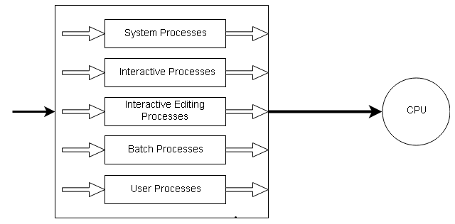
Another option is to time-slice the queues. Each queue gets a certain percent of the CPU time. If the priority is high it will be given more time and the lower queue will get less CPU time.

Multilevel Feedback Queue

There is another version of the multilevel queue called the multilevel feedback queue which allows a process to move between queues. If the process uses too much of CPU time, it is moved to a lower-priority queue. If the process starts aging (waits too much in a lower-priority queue) is moved to a higher-priority queue. This prevents the process from starvation.

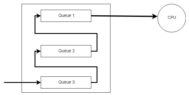
Figure 2 – Multilevel Feedback Queue

The following properties define the multilevel feedback queue:

– The number of queues
– The scheduling algorithm for each queue
– The method for upgrading the process from lower-priority queue to higher-priority queue.
– The method for downgrading the process from higher-priority queue to lower-priority queue.
– The method to determine the queue in which process will enter.

Basically, the multilevel feedback queue seems very general CPU scheduling algorithm. However, it is quite complex to design and implement a multilevel feedback queue.

References

Abraham Silberschatz, Peter B. Galvin, Greg Gagne (July 29, 2008) Operating System Concepts, 8 edn., : Wiley.
Tanenbaum, Andrew S. (March 3, 2001) Modern Operating Systems, 2nd edn., : Prentice Hall.

post

Fork-Join Concept

The fork-join is a basic method of expressing concurrency within a computation. This is implemented in the UNIX operating system as system calls.

Fork

The fork() call creates a new child process which runs concurrently with the parent. The child process is an exact copy of the parent except that it has a new process id. The fork() creates concurrency.

Join

The join() is called by both the parent and the child. The child process calls join() after it has finished execution. This operation is done implicitly. The parent process waits until the child joins and continues later.

The join() call breaks the concurrency because the child process exits. The join() inform the parent that child operation is finished.

There are two join scenarios:

The child joins first and then the parent joins without waiting for any process.
The parent process joins first and wait, the child process joins, and the parent continues thereafter.

Example #1

The parent executes “fork L” statement. It creates a child process which runs concurrently- one process (parent) continues after the fork operation and other (child) statement runs at statement labeled L.

S1;

fork L;

S2     /* Statement right after fork operation */

...

...

L: S3     /* statement labeled L */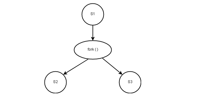

Figure 1 – Fork-Join Precedence Graph

The fork splits the single operation into two independent operation – S2 and S3.

The join call combines the two concurrent process into one. The process which executes join first will be terminated and the other process continues. If it is parent S2 that terminates first, then it will wait for S3 to finish.

Figure 2 – Join () Precedence Graph

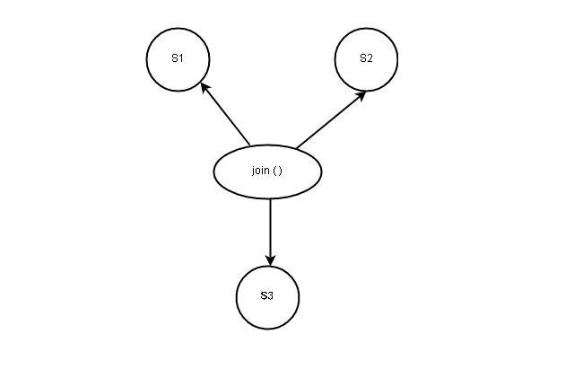
If S3 join first, then S2 will join later after finishing the execution without waiting.

post

Concurrency Conditions

There are certain conditions for concurrency. Here we have listed them for you in this article.

Conditions for Concurrency

$R(S_i) = \{ a_1, a_2, a_3, \cdots , a_m \}$ , the read set for $S_i$ , is the set of all variables whose values are referenced in statement $S_i$ during its execution.

$W(S_i) = \{b_1, b_2, b_3, \cdots, b_n \}$ , the write set for $S_i$ , is the set of all variables whose values are changed or written by the execution of statement $S_i$ .

Example #1

Consider the statement.

$C:= A - B$

The read set:

$R(C:= A - B) = \{A, B\}$

The write set:

$W(C:= A - B) = \{C\}$

The intersection of $R(S_i)$ and $W(S_i)$ need not be null.

Example #2

Consider following statement:

$X:= X + 2$

The read set:

$R(X:= X + 2) = \{ X \}$

The write set:

$W(X:= X + 2) = \{ X \}$

Bernstein’s Conditions

The following three conditions must be satisfied for two successive statements $S_i$ and $S_j$ to be executed concurrently and still produce the same results known as Bernstein’s conditions.

$R(S_1) \cap W(S_2)= \{ \}$ .
$W(S_1) \cap R(S_2) = \{ \}$ .
$W(S_1) \cap W(S_2) = \{ \}$ .

Example:

Consider the following statements.

$S_1: a:=x-y$ .
$S_2: b:=z-1$ .

$R(S_1) = \{ x, y \}$ .
$R(S_2) = \{ z \}$ .
$W(S_1) = \{ a \}$ .
$W(S_2) = \{ b \}$ .

In the example above, all three conditions are satisfied. Therefore, the statement $S_1$ and $S_2$ can be executed concurrently.

We could use the precedence graph, but the precedence graph cannot be used in programming as it is a two-dimensional object. Moreover, it only shows the dependency relationship between statements.

post